Difference between revisions of "SOCR EduMaterials AnalysisActivities MLR"
(→SOCR Multiple Linear Regression Data Input) |
m (→See also) |
||
| (7 intermediate revisions by 2 users not shown) | |||
| Line 21: | Line 21: | ||
==SOCR Multiple Linear Regression Data Input== | ==SOCR Multiple Linear Regression Data Input== | ||
| − | Go to SOCR Analyses and select '''Multiple Linear Regression''' from the drop-down list of SOCR analyses, in the left panel. There are three ways to enter data in the SOCR Multiple Linear Regression applet: | + | Go to [http://www.socr.ucla.edu/htmls/ana/MultipleRegression_Analysis.html SOCR Analyses and select '''Multiple Linear Regression'''] from the drop-down list of SOCR analyses, in the left panel. There are three ways to enter data in the SOCR Multiple Linear Regression applet: |
* Click on the '''Example''' button on the top of the right panel. | * Click on the '''Example''' button on the top of the right panel. | ||
* Generate random data by clicking on the '''Random Example''' button. | * Generate random data by clicking on the '''Random Example''' button. | ||
* Paste your own data from a spreadsheet into SOCR Multiple Linear Regression data table. | * Paste your own data from a spreadsheet into SOCR Multiple Linear Regression data table. | ||
| + | ==SOCR Multiple Linear Regression Example== | ||
| + | We will demonstrate Multiple Linear Regression with some SOCR built-in example. This example is based on a dataset from the statistical program "R." For more information of the R program, please see [http://cran.r-project.org/ CRAN Home Page]. The dataset used here is "hills" under R's "MASS" library. The dataset describe the record times in 1984 for 35 Scottish hill races. There are three variables: '''dist''' for distance in miles, '''climb''' total height gained during the route, in feet, and '''time''' record time in minutes. In our example, we will use '''time''' as the dependent variable, and '''climb''' and '''dist''' as the independent variables. | ||
| − | + | ||
| − | + | * As you start the SOCR Analyses Applet, click on "'''Multiple Linear Regression'''" from the combo box in the left panel. Here's what the screen should look like. | |
| + | <center>[[Image:SOCR_AnalysisActivities_MLR_Chu_072607_Fig1.gif|800px]]</center> | ||
| + | |||
| + | |||
| + | * The left part of the panel looks like this (make sure that the "Multiple Linear Regression" is showing in the drop-down list of analyses, otherwise you won't be able to find the correct dataset and will not be able to reproduce the results!) | ||
| + | <center>[[Image:SOCR_AnalysisActivities_MLR_Chu_051707_Fig4.gif|450px]]</center> | ||
| + | |||
| + | |||
| + | * in the SOCR MLR analysis, there are several SOCR built-in examples. In this activity, we'll be using '''Example 4'''. Click on the "'''Example 4'''" button and next, click on the "'''Data'''" button in the right panel. You should see the data displayed in two columns. There are three columns here, '''dist''', '''climb''' and '''time'''. | ||
| + | <center>[[Image:SOCR_AnalysisActivities_MLR_Chu_051707_Fig1.gif|700px]]</center> | ||
| + | |||
| + | |||
| + | * Use column '''dist''' and '''climb''' as the regressors (independent variables) and column '''time''' as the response (dependent variable). To tell the computer which variables are assigned to be the regressor and response, we have to do a "Mapping." This is done by clicking on the "'''Mapping'''" button first to get to the Mapping Panel, and then map the variables. For this Multiple Linear Regression activity, there are two places the variables can be mapped to. The top part says '''DEPENDENT''' that you'll need to '''map''' the dependent variable you want here. Just click on '''ADD''' under '''DEPENDENT''' and that will do it. If you change your mind, you can click on '''REMOVE'''. Similar for the '''INDEPENDENT''' variable. Once you get the screen to look like the screenshot below, you're done with the '''Mapping''' step. (Note that, since the columns C4 through C16 do not have data and they are not used, just ignore them.) | ||
| + | <center>[[Image:SOCR_AnalysisActivities_MLR_Chu_051707_Fig2.gif|700px]]</center> | ||
| + | |||
| + | |||
| + | * After we do the "Mapping" to assign variables, now we use the computer to calculate the regression results -- click on the "'''Calculate'''" button. Then select the "'''Result'''" panel to see the output. For each of the coefficients, '''Estimate''' stands for the estimated parameter value, followed by its '''Standard Error''', '''T-Value''' and '''P-Value'''. | ||
| + | <center>[[Image:SOCR_AnalysisActivities_MLR_Chu_051707_Fig6.gif|700px]]</center> | ||
| + | |||
| + | The text in the Result Panel summarizes the results of this simple linear regression analysis. The regression line is displayed. At this point, you can think about how the '''dependent variable''' changes, on average, in response to changes of the '''independent variable'''. | ||
| + | |||
| + | |||
| + | * If you'd like to see graphical component of this analysis, click on the "'''Graph'''" panel. You'll then see the graph panel that displays scatter plot, as well as diagnostic plots of "residual on fit", "Normal QQ" plots, etc. The plot titles indicate plot types. | ||
| + | |||
| + | |||
| + | <center>[[Image:SOCR_AnalysisActivities_MLR_Chu_051707_Fig7.gif|700px]]</center> | ||
| + | |||
| + | |||
| + | <center>[[Image:SOCR_AnalysisActivities_MLR_Chu_051707_Fig5.gif|700px]]</center> | ||
| + | |||
| + | |||
| + | <center>[[Image:SOCR_AnalysisActivities_MLR_Chu_051707_Fig3.gif|700px]]</center> | ||
| + | |||
| + | |||
| + | <center>[[Image:SOCR_AnalysisActivities_MLR_Chu_051707_Fig8.gif|700px]]</center> | ||
| + | |||
| + | |||
| + | <center>[[Image:SOCR_AnalysisActivities_MLR_Chu_051707_Fig9.gif|700px]]</center> | ||
| + | |||
| + | |||
| + | <center>[[Image:SOCR_AnalysisActivities_MLR_Chu_051707_Fig10.gif|700px]]</center> | ||
| + | |||
| + | |||
| + | |||
| + | '''Note''': If you happen to click on the "'''Clear'''" button in the middle of the procedure, '''all the data will be cleared out'''. Simply start over from step 1 and click on an '''EXAMPLE''' button for the data you want. | ||
| + | |||
| + | ==Assumptions== | ||
| + | The SOCR MLR analysis implements the [http://en.wikipedia.org/wiki/General_linear_model General Linear Model (GLM)] and does *not* require normality. Only the [http://en.wikipedia.org/wiki/Linear_regression#Assumptions 2 assumptions] listed are: | ||
| + | * The design matrix X must have full column rank, otherwise the parameter vector β will not be identified — at most we will be able to narrow down its value to some linear subspace of <math>{R}^p</math>. For this property to hold, we must have n > p, where n is the sample size, and p is the column rank. Methods for fitting. | ||
| + | * The regressors <math>X_i</math> are assumed to be error-free, that is they are not contaminated with measurement errors. Although not realistic in many settings, dropping this assumption leads to significantly more difficult errors-in-variables models. | ||
| + | |||
| + | ==See also== | ||
| + | [[SOCR_EduMaterials_AnalysesCommandLineVolumeMultipleRegression|Command-line based multiple linear regression execution]]. | ||
| + | |||
| + | <hr> | ||
| + | |||
| + | {{translate|pageName=http://wiki.stat.ucla.edu/socr/index.php?title=SOCR_EduMaterials_AnalysisActivities_MLR}} | ||
Latest revision as of 12:08, 24 September 2012
Contents
SOCR Analysis Example on Multiple Linear Regression
This SOCR Activity demonstrates the utilization of the SOCR Analyses package for statistical Computing. In particular, it shows how to use Multiple Linear Regression and how to read the output results.
Multiple Linear Regression Background
Multiple Linear Regression is a class of statistical analysis models and procedures, which takes one independent variable and one dependent and one or more variable, both sets being quantitative, and models the relationship between them. SOCR has another activity set for Simple Linear Regression, which only allows on independent variable in the input. However, SOCR Multiple Linear Regression allows one or more independent variables. In the linear model, the error is assumed to follow a standard normal distribution.
The goal of the Multiple Linear Regression computing procedure is to estimate all of the coefficients based on the data. Least Squares Fitting is used.
In this activity, the students can learn about:
- Reading results of Simple Linear Regression;
- Making interpretation of the coefficients;
- Observing and interpreting various data and resulting plots
- Scatter plots of the dependent vs. independent variables
- Diagnostic plots such as the Residual on Fit plot
- Normal QQ plot, etc.
SOCR Multiple Linear Regression Data Input
Go to SOCR Analyses and select Multiple Linear Regression from the drop-down list of SOCR analyses, in the left panel. There are three ways to enter data in the SOCR Multiple Linear Regression applet:
- Click on the Example button on the top of the right panel.
- Generate random data by clicking on the Random Example button.
- Paste your own data from a spreadsheet into SOCR Multiple Linear Regression data table.
SOCR Multiple Linear Regression Example
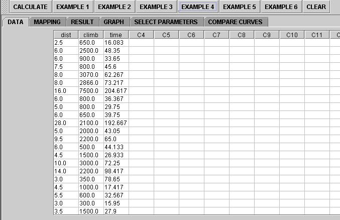
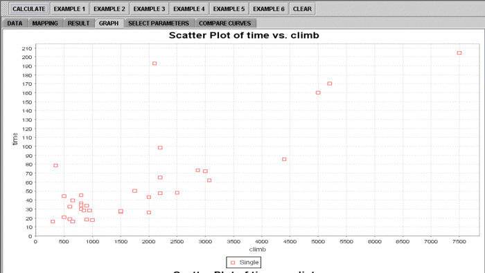
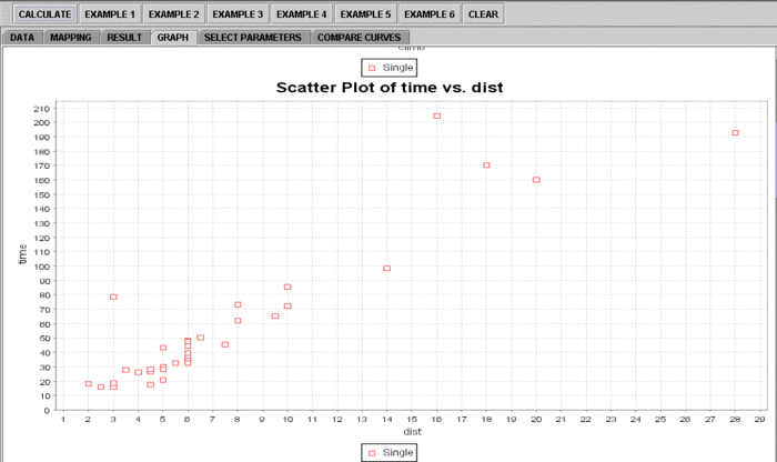
We will demonstrate Multiple Linear Regression with some SOCR built-in example. This example is based on a dataset from the statistical program "R." For more information of the R program, please see CRAN Home Page. The dataset used here is "hills" under R's "MASS" library. The dataset describe the record times in 1984 for 35 Scottish hill races. There are three variables: dist for distance in miles, climb total height gained during the route, in feet, and time record time in minutes. In our example, we will use time as the dependent variable, and climb and dist as the independent variables.
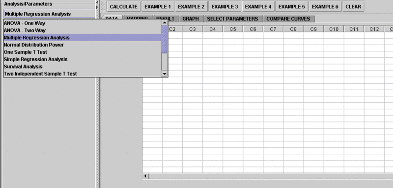
- As you start the SOCR Analyses Applet, click on "Multiple Linear Regression" from the combo box in the left panel. Here's what the screen should look like.
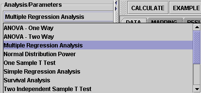
- The left part of the panel looks like this (make sure that the "Multiple Linear Regression" is showing in the drop-down list of analyses, otherwise you won't be able to find the correct dataset and will not be able to reproduce the results!)
- in the SOCR MLR analysis, there are several SOCR built-in examples. In this activity, we'll be using Example 4. Click on the "Example 4" button and next, click on the "Data" button in the right panel. You should see the data displayed in two columns. There are three columns here, dist, climb and time.
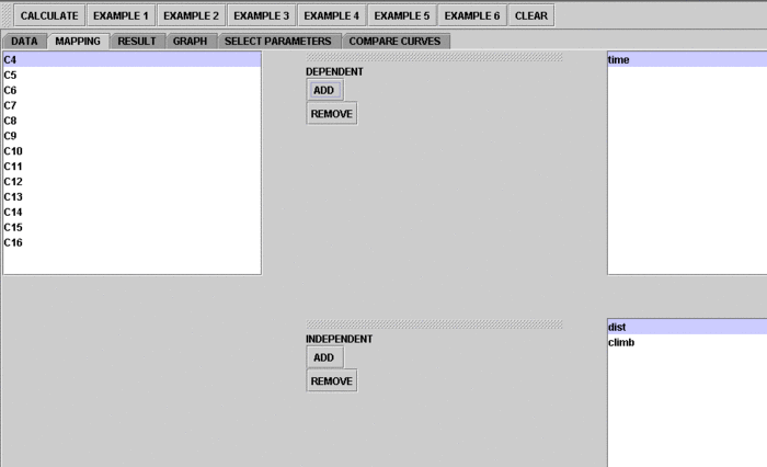
- Use column dist and climb as the regressors (independent variables) and column time as the response (dependent variable). To tell the computer which variables are assigned to be the regressor and response, we have to do a "Mapping." This is done by clicking on the "Mapping" button first to get to the Mapping Panel, and then map the variables. For this Multiple Linear Regression activity, there are two places the variables can be mapped to. The top part says DEPENDENT that you'll need to map the dependent variable you want here. Just click on ADD under DEPENDENT and that will do it. If you change your mind, you can click on REMOVE. Similar for the INDEPENDENT variable. Once you get the screen to look like the screenshot below, you're done with the Mapping step. (Note that, since the columns C4 through C16 do not have data and they are not used, just ignore them.)
- After we do the "Mapping" to assign variables, now we use the computer to calculate the regression results -- click on the "Calculate" button. Then select the "Result" panel to see the output. For each of the coefficients, Estimate stands for the estimated parameter value, followed by its Standard Error, T-Value and P-Value.
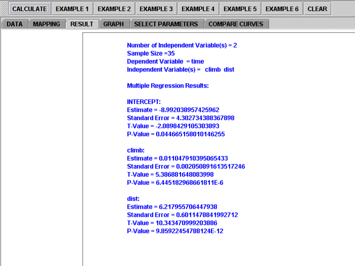
The text in the Result Panel summarizes the results of this simple linear regression analysis. The regression line is displayed. At this point, you can think about how the dependent variable changes, on average, in response to changes of the independent variable.
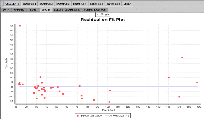
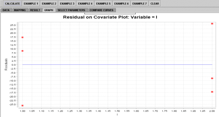
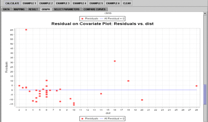
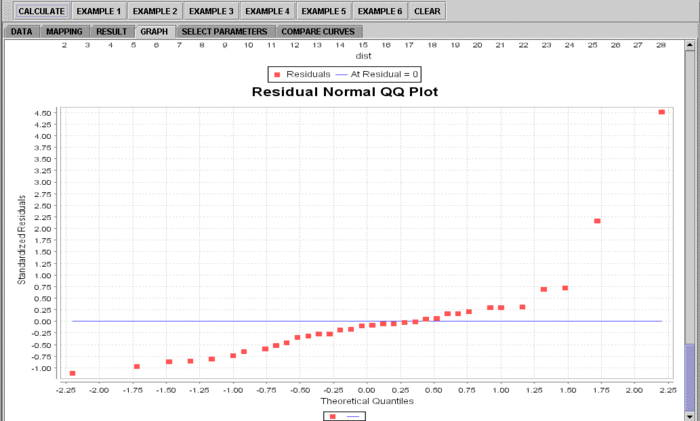
- If you'd like to see graphical component of this analysis, click on the "Graph" panel. You'll then see the graph panel that displays scatter plot, as well as diagnostic plots of "residual on fit", "Normal QQ" plots, etc. The plot titles indicate plot types.
Note: If you happen to click on the "Clear" button in the middle of the procedure, all the data will be cleared out. Simply start over from step 1 and click on an EXAMPLE button for the data you want.
Assumptions
The SOCR MLR analysis implements the General Linear Model (GLM) and does *not* require normality. Only the 2 assumptions listed are:
- The design matrix X must have full column rank, otherwise the parameter vector β will not be identified — at most we will be able to narrow down its value to some linear subspace of \({R}^p\). For this property to hold, we must have n > p, where n is the sample size, and p is the column rank. Methods for fitting.
- The regressors \(X_i\) are assumed to be error-free, that is they are not contaminated with measurement errors. Although not realistic in many settings, dropping this assumption leads to significantly more difficult errors-in-variables models.
See also
Command-line based multiple linear regression execution.
Translate this page: