Difference between revisions of "SMHS TimeSeriesAnalysis"
(→Scientific Methods for Health Sciences - Time Series Analysis) |
(→Scientific Methods for Health Sciences - Time Series Analysis) |
||
| Line 247: | Line 247: | ||
[[Image:SMHS_TimeSeries7.png|500px]] | [[Image:SMHS_TimeSeries7.png|500px]] | ||
| + | |||
| + | <b>Plot the trend on the observed data -- with prediction:</b> | ||
| + | |||
| + | pred2 <- predict(mod$\$$gam, newdata = l.sort, type = "terms") | ||
| + | |||
| + | ptemp2 <- attr(pred2, "constant") + <u>pred2[,1]</u> | ||
| + | |||
| + | <b># pred2[,1] = trend; pred2[,2] = seasonal effects</b> | ||
Revision as of 10:20, 6 May 2016
Scientific Methods for Health Sciences - Time Series Analysis
Questions
• Why are trends, patterns or predictions from models/data important?
• How to detect, model and utilize trends in longitudinal data?
Time series analysis represents a class of statistical methods applicable for series data aiming to extract meaningful information, trend and characterization of the process using observed longitudinal data. These trends may be used for time series forecasting and for prediction of future values based on retrospective observations. Note that classical linear modeling (e.g., regression analysis) may also be employed for prediction & testing of associations using the values of one or more independent variables and their affect the value of another variable. However, time series analysis allows dependencies (e.g., seasonal effects to be accounted for).
Time-series representation
There are 3 (distinct and complementary) types of time series patterns that most time-series analyses are trying to identify, model and analyze. These include:
• Trend: A trend is a long-term increase or decrease in the data that may be linear or non-linear, but is generally continuous (mostly monotonic). The trend may be referred to as direction.
• Seasonal: A seasonal pattern is influence in the data, like seasonal factors (e.g., the quarter of the year, the month, or day of the week), which is always of a fixed known period.
• Cyclic: A cyclic pattern of fluctuations corresponds to rises and falls that are not of fixed period.
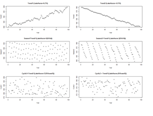
For example, the following code shows several time series with different types of time series patterns.
par(mfrow=c(3,2))
n <- 98
X <- cbind(1:n)   # time points (annually)
Trend1 <- LakeHuron+0.2*X  # series 1
Trend2 <- LakeHuron-0.5*X  # series 2
Season1 <- X; Season2 <- X;  # series 1 & 2
for(i in 1:n) {
Season1[i] <- LakeHuron[i] + 5*(i%%4)
Season2[i] <- LakeHuron[i] -2*(i%%10)
}
Cyclic1 <- X; Cyclic2 <- X;  # series 1 & 2
for(i in 1:n) {
rand1 <- as.integer(runif(1, 1, 10))
Cyclic1[i] <- LakeHuron[i] + 3*(i%%rand1)
Cyclic2[i] <- LakeHuron[i] - 1*(i%%rand1)
}
plot(X, Trend1, xlab="Year",ylab=" Trend1", main="Trend1 (LakeHuron+0.2*X)")
plot(X, Trend2, xlab="Year",ylab=" Trend2" , main="Trend2 (LakeHuron-0.5*X)")
plot(X, Season1, xlab="Year",ylab=" Season1", main=" Season1=Trend1 (LakeHuron+5(i%%4))")
plot(X, Season2, xlab="Year",ylab=" Season2", main=" Season2=Trend1 (LakeHuron-2(i%%10))")
plot(X, Cyclic1, xlab="Year",ylab=" Cyclic1", main=" Cyclic1=Trend1 (LakeHuron+3*(i%%rand1))")
plot(X, Cyclic2, xlab="Year",ylab=" Cyclic2", main=" Cyclic2 = Trend1 (LakeHuron-(i%%rand1))")
Note: If you get this run-time graphics error: “Error in plot.new() : figure margins too large”
You need to make sure your graphics window is large enough or print to PDF:
pdf("myplot.pdf"); plot(x); dev.off()
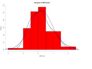
Let’s look at the delta (Δ) changes - Lagged Differences, using diff, which returns suitably lagged and iterated differences.
- Default lag = 1
par(mfrow=c(1,1))
hist(diff(Trend1), prob=T, col="red") # Plot histogram
lines(density(diff(Trend1)),lwd=2) # plot density estimate
x<-seq(-4,4,length=100); y<-dnorm(x, mean(diff(Trend1)), sd(diff(Trend1)))
lines(x,y,lwd=2,col="blue") # plot MLE Normal Fit
Time series decomposition
Denote the time series yt including the three components: a seasonal effect, a trend-cycle effect (containing both trend and cycle), and a remainder component (containing the residual variability in the time series).
Additive model: yt=St+Tt+Et, where yt is the data at period t, St is the seasonal component at period t, Tt is the trend-cycle component at period t and Et is the remainder (error) component at period t. This additive model is appropriate if the magnitude of the seasonal fluctuations or the variation around the trend-cycle does not vary with the level of the time series.
Multiplicative model: yt=St×Tt×Et. When the variation in the seasonal pattern, or the variation around the trend-cycle, are proportional to the level of the time series, then a multiplicative model is more appropriate. Note that when using a multiplicative model, we can transform the data to stabilize the variation in the series over time, and then use an additive model. For instance, a log transformation decomposes the multiplicative model from:
yt=St×Tt×Et
to the additive model:
log(yt)=log(St)+log(Tt)+log(Et).
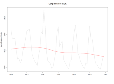
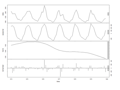
We can examine the Seasonal trends by decomposing the Time Series by loess (Local Polynomial Regression) Fitting into Seasonal, Trend and irregular components using Loess - Local Polynomial Regression Fitting (stl function, in the default “stats” package):
# using Monthly Males Deaths from Lung Diseases in UK from bronchitis, emphysema and asthma, 1974–1979 mdeaths # is.ts(mdeaths)
fit <- stl(mdeaths, s.window=5)
plot(mdeaths, col="gray", main=" Lung Diseases in UK ", ylab=" Lung Diseases Deaths", xlab="")
lines(fit$time.series[,2],col="red",ylab="Trend")
plot(fit) # data, seasonal, trend, residuals
|
x||Univariate time series to be decomposed. This should be an object of class "ts" with a frequency greater than one. | |
|---|---|
| s.window | either the character string "periodic" or the span (in lags) of the loess window for seasonal extraction, which should be odd and at least 7, according to Cleveland et al. This has no default. |
| s.degree | degree of locally-fitted polynomial in seasonal extraction. Should be zero or one. |
| t.window | the span (in lags) of the loess window for trend extraction, which should be odd. If NULL, the default, nextodd(ceiling((1.5*period) / (1-(1.5/s.window)))), is taken. |
| t.degree | degree of locally-fitted polynomial in trend extraction. Should be zero or one. |
| l.window | the span (in lags) of the loess window of the low-pass filter used for each subseries. Defaults to the smallest odd integer greater than or equal tofrequency(x) which is recommended since it prevents competition between the trend and seasonal components. If not an odd integer its given value is increased to the next odd one. |
| l.degree | degree of locally-fitted polynomial for the subseries low-pass filter. Must be 0 or 1. |
| s.jump, t.jump, l.jump | integers at least one to increase speed of the respective smoother. Linear interpolation happens between every *.jumpth value. |
| robust | logical indicating if robust fitting be used in the loess procedure. |
| inner | integer; the number of ‘inner’ (backfitting) iterations; usually very few (2) iterations suffice. |
| outer | integer; the number of ‘outer’ robustness iterations. |
| na.action | action on missing values. |
monthplot(fit$\$$time.series[,"seasonal"], main="", ylab="Seasonal", lwd=5) # As the “fit <- stl(mdeaths, s.window=5)” object has 3 time-series components (seasonal; trend; remainder) # we can alternatively plot them separately: # monthplot(fit, choice = <b><u>"seasonal"</u></b>, cex.axis = 0.8) # monthplot(fit, choice = <b><u>"trend"</u></b>, cex.axis = 0.8) # monthplot(fit, choice = <b><u>"remainder"</u></b>, type = "h", cex.axis = 1.2) # histogramatic [[Image:SMHS_TimeSeries5.png|400px]] These are the seasonal plots and seasonal sub-series plots of the seasonal component illustrating the variation in the seasonal component over time (over the years). Using historical weather (average daily temperature at the University of Michigan, Ann Arbor): [http://weather-warehouse.com/WeatherHistory/PastWeatherData_AnnArborUnivOfMi_AnnArbor_MI_January.html] (See meta-data description and provenance online: [http://weather-warehouse.com/WxWfaqs.html]). <b><center>Mean Temperature, (F), UMich, Ann Arbor (1900-2015)</center></b> <center> {| class="wikitable" style="text-align:center; " border="1" |- !Year||Jan||Feb||Mar||Apr||May||Jun||Jul||Aug||Sep||Oct||Nov||Dec |- |2015||26.3||14.4||34.9||49||64.2||68||71.2||70.2||68.7||53.9||NR||NR |- |2014||24.4||19.4||29||48.9||60.7||69.7||68.8||70.8||63.2||52.1||35.4||33.3 |- |2013||22.7||26.1||33.3||46||63.1||68.5||72.9||70.2||64.6||53.2||37.6||26.7 |- |2012||22.4||32.8||50.7||49.2||65.2||71.4||78.9||72.2||63.9||51.7||39.6||34.8 |- |...|| || || || || || || || || || || || || |- |...||17||15.3||31.4||47.3||57||69||76.6||72||63.4||52.2||35.2||23.7 |- |1900||21.4||19.2||24.7||47.8||60.2||66.3||72||75.4||67.2||59||37.6||29.2 |} </center> # data: 07_UMich_AnnArbor_MI_TempPrecipitation_HistData_1900_2015.csv # more complete data is available here: 07_UMich_AnnArbor_MI_TempPrecipitation_HistData_1900_2015.xls umich_data <- read.csv("https://umich.instructure.com/files/702739/download?download_frd=1", header=TRUE) head(umich_data) # https://cran.r-project.org/web/packages/mgcv/mgcv.pdf # install.packages("mgcv"); require(mgcv) # install.packages("gamair"); require(gamair) par(mfrow=c(1,1)) The data are in wide format – convert to long format for plotting # library("reshape2") long_data <- melt(umich_data, id.vars = c("Year"), value.name = "temperature") l.sort <- long_data[order(long_data$\$$Year),]
head(l.sort); tail(l.sort)
plot(l.sort$\$$temperature, data = l.sort, type = "l") <b>Fit the GAMM Model</b> (Generalized Additive Mixed Model) [[Image:SMHS_TimeSeries6.png|400px]] <b>Fit a model with trend and seasonal components</b> --- computation may be slow: # define the parameters controlling the process of model-fitting/parameter-estimation ctrl <- list(niterEM = 0, msVerbose = TRUE, optimMethod="L-BFGS-B") # First try this model mod <- gamm(as.numeric(temperature) ~ s(as.numeric(Year)) + s(as.numeric(variable)), data = l.sort, method = "REML", correlation=corAR1(form = ~ 1|Year), knots=list(Variable = c(1, 12)), na.action=na.omit, control = ctrl) # <u>Correlation</u>: <b>corStruct</b> object defineing correlation structures in <b>lme</b>. Grouping factors in the formula for this # object are assumed to be nested within any random effect grouping factors, without the need to make this # explicit in the formula (somewhat different from the behavior of <b>lme</b>). # This is similar to the GEE approach to correlation in the generalized case. # <u>Knots</u>: an optional list of user specified knot values to be used for basis construction -- # different terms can use different numbers of knots, unless they share a covariate. # If you revise the model like this (below), it will compare nicely with 3 ARMA models (later) mod <- gamm(as.numeric(temperature) ~ s(as.numeric(Year), k=116) + s(as.numeric(variable), k=12), data = l.sort, correlation = corAR1(form = ~ 1|Year), control = ctrl) <b>Summary of the fitted model:</b> summary(mod$\$$gam)
Visualize the model trend (year) and seasonal terms (months)
plot(mod$\$$gam, pages = 1) t <- cbind(1: 1392) # define the time [[Image:SMHS_TimeSeries7.png|500px]] <b>Plot the trend on the observed data -- with prediction:</b> pred2 <- predict(mod$\$$gam, newdata = l.sort, type = "terms")
ptemp2 <- attr(pred2, "constant") + pred2[,1]
# pred2[,1] = trend; pred2[,2] = seasonal effects


