Difference between revisions of "EBook Problems MultivariateNormal"
(→EBook Problems Set - Mutivariate Normal Distribution) |
m (Text replacement - "{{translate|pageName=http://wiki.stat.ucla.edu/socr/" to ""{{translate|pageName=http://wiki.socr.umich.edu/") |
||
| (6 intermediate revisions by one other user not shown) | |||
| Line 294: | Line 294: | ||
\Rightarrow\sigma_x=\sqrt{300} \cong 17.32(m^3/sec) \, | \Rightarrow\sigma_x=\sqrt{300} \cong 17.32(m^3/sec) \, | ||
</math> | </math> | ||
| + | }} | ||
| + | {{hidden|Answer for part (b)| | ||
| + | The annual risk of flooding, <math>p=P(X>100) \,</math> | ||
| + | <math> | ||
| + | =P(\frac{X-\mu_x}{\sigma_x}>\frac{100-60}{\sqrt{300}}) \, | ||
| + | </math> | ||
| + | |||
| + | <math> | ||
| + | =1-\Phi(2.309401077)=1-0.989539359 \, | ||
| + | </math> | ||
| + | |||
| + | <math> | ||
| + | \cong 0.0105 \,</math> (probability each year) | ||
| + | |||
| + | Hence the return period is: | ||
| + | |||
| + | <math> | ||
| + | \tau=\frac{1}{p} \, | ||
| + | </math> | ||
| + | |||
| + | <math> | ||
| + | =\frac{1}{0.010460641}=95.59643882 \, | ||
| + | </math> | ||
| + | |||
| + | <math> | ||
| + | \cong 96 years \, | ||
| + | </math> | ||
| + | }} | ||
| + | {{hidden|Answer for part (c)| | ||
| + | Since the yearly risk of flooding is <math>p=0.010460641</math>, and we have a course of <math>n=10</math> years, we adopt a binomial model for Y, the total number of flood years over a 10-year period. | ||
| + | |||
| + | P(city experiences (any) flooding)<math>=</math> 1-P(city experiences no flooding at all) | ||
| + | |||
| + | <math> | ||
| + | = 1-P(Y=0) | ||
| + | </math> | ||
| + | |||
| + | <math> | ||
| + | =1-(1-p)^{10}=1-(1-0.010460641)^{10} | ||
| + | </math> | ||
| + | |||
| + | <math> | ||
| + | =1-0.989539359^{10}=1-0.900182843 | ||
| + | </math> | ||
| + | |||
| + | <math> | ||
| + | \cong 10% | ||
| + | </math> | ||
}} | }} | ||
| + | {{hidden|Answer for part (d)| | ||
| + | The requirement on p is, using the flooding probability expression from part (c): | ||
| + | |||
| + | <math> | ||
| + | 1-(1-p)^{10}=\frac{0.099817157}{2}=0.049908579 | ||
| + | </math> | ||
| + | |||
| + | <math> | ||
| + | \Rightarrow p=1-(1-0.49908579)^{1/10}=0.005106623 | ||
| + | </math> | ||
| + | |||
| + | This translates into a condition on the design channel capacity <math>X_0</math>, following what's done in (b), | ||
| + | |||
| + | <math> | ||
| + | P(\frac{X-\mu_x}{\sigma_x}>\frac{X_0-60}{\sqrt{300}})=p | ||
| + | </math> | ||
| + | |||
| + | <math> | ||
| + | \Rightarrow 1-\Phi(\frac{X_0-60}{\sqrt{300}})=0.005106623 | ||
| + | </math> | ||
| + | |||
| + | <math> | ||
| + | \Rightarrow \Phi((\frac{X_0-60}{\sqrt{300}}))=0.994893377 | ||
| + | </math> | ||
| + | |||
| + | <math> | ||
| + | \Rightarrow X_0=60+\Phi^{-1}(0.994893377)\sqrt{300} | ||
| + | </math> | ||
| + | |||
| + | <math> | ||
| + | =60+2.568522177 \sqrt{300} = 104.4881091 | ||
| + | </math> | ||
| + | |||
| + | Therefore, extending the channel capacity to about <math>104.5</math> <math>m^3/sec</math> will cut the risk by half. | ||
| + | }} | ||
| + | |||
| + | ===Problem 5=== | ||
| + | Fibers may be embedded in cement to increase its strength. Consider a cracked section as shown in the following diagram: | ||
| + | |||
| + | [[Image:Problem 5.jpg|250x250px|center]] | ||
| + | |||
| + | Suppose the total strength T of the cracked section is given by the following expression: | ||
| + | |||
| + | <math> | ||
| + | T=C+(F_1+F_2+...+F_N) | ||
| + | </math> | ||
| + | |||
| + | Where C is the strength contributed by the cement; <math>F_1</math>, <math>F_2</math>, etc. are the strength of each of the fibers across the crack; N is the total number of fibers across the crack. Suppose C=N(30,5); each <math>F_i</math> is N(5,3) and N is a discrete random variable with the following PMF | ||
| + | |||
| + | |||
| + | [[Image:Problem 5 PMF.jpg|600x600px|center]] | ||
| + | |||
| + | Assume C and <math>F_i</math>'s are statistically independent. What is the probability that the total strength T will be less than 30? | ||
| + | |||
| + | ===Problem 6=== | ||
| + | [[Image:Problem 6.jpg|300x300px|center]] | ||
| + | |||
| + | The settlement of each footing shown follows a normal distribution with a mean of 2 inches and a coefficient of variation of 30%. Suppose the settlements between two adjacent footings are correlated with a correlation coefficient of 0.7. suppose | ||
| + | |||
| + | <math>D=S_1-S_2</math> | ||
| + | |||
| + | where <math>S_1</math> and <math>S_2</math> are settlements of footings 1 and 2, respectively. | ||
| + | |||
| + | ''(a) Determine the mean and variance of D. | ||
| + | |||
| + | ''(b) What is the probability that the magnitude of the differential settlement (i.e., the difference between the settlements of two adjacent footings) will be less than 0.5 inch? | ||
| + | |||
| + | ===Problem 7=== | ||
| + | [[Image:Problem 7.jpg|600x600px|center]] | ||
| + | |||
| + | The systems of pipes shown in the figure is supposed to carry the storm runoffs <math>X_1</math> and <math>X_2</math>, and the municipal waste water, <math>X_3</math>. Suppose the statistics of the flow rates (all in units of cubic feet per second, CFS) are: | ||
| + | |||
| + | {| border="1" align="center" | ||
| + | |- | ||
| + | ! scope="col" | | ||
| + | ! scope="col" | Mean | ||
| + | ! scope="col" | c.o.v. | ||
| + | ! scope="col" | Distribution | ||
| + | |- | ||
| + | ! scope="row" | <math>X_1</math> | ||
| + | | 10 || 0.3 || Normal | ||
| + | |- | ||
| + | ! scope="row" | <math>X_2</math> | ||
| + | | 15 || 0.2 || Normal | ||
| + | |- | ||
| + | ! scope="row" | <math>X_3</math> | ||
| + | | 20 || 0.00 || --- | ||
| + | |} | ||
| + | |||
| + | |||
| + | Because of proximity, <math>X_1</math> and <math>X_2</math> are dependent. Assume that the coefficient of correlation <math>\rho_{X_1,X_2}=0.6</math>. | ||
| + | |||
| + | ''(a) Determine the mean value and standard deviation of the total rate of inflow to pipe 5. | ||
| + | |||
| + | ''(b) What is the probability that during a '''one minute interval''', the volume of water flowing into pipe 2 exceeds that into pipe 1 by at least 400 cubic feet? (Hint: assume the inflow rate into each pipe is constant during that minute) | ||
| + | |||
| + | ''(c) Suppose the municipal waste water is projected to increase at a rate of 3 cfs per year, and pipe 5 has a capacity of 70 cfs. If the design criterion is that the probability of overflow at pipe 5 (total inflow exceeds capacity) after a storm should be less than 0.05, how many years will the current pipe 5 remain adequate, i.e., before a larger size pipe is needed? | ||
| + | |||
| + | ===Problem 8=== | ||
| + | The flows in two tributaries 1 and 2 combine to form stream 3 as shown in the following figure: | ||
| + | |||
| + | [[Image:Problem 8.jpg|400x400px|center]] | ||
| + | |||
| + | Suppose the concentration of pollutants in tributary 1 is X which is normally distributed as N(20,4) parts per unit volume (puv); whereas that in tributary 2 is Y which is N(15,3) puv. The flow rate in tributary 1 is 600 puv cubic feet per sec (cfs) and that in 2 is 400 cfs. Hence the concentration of pollutants in the stream is | ||
| + | |||
| + | <math> | ||
| + | Z=\frac{600X+400Y}{600+400}=0.6X+0.4Y | ||
| + | </math> | ||
| + | |||
| + | Pollution occurs if pollutant concentration exceeds 20 puv. | ||
| + | |||
| + | ''(a) What is the probability that '''at least one''' of the two tributaries will be polluted? | ||
| + | |||
| + | ''(b) Assume X and Y are statistically independent. Determine the probability of a polluted stream? | ||
| + | |||
| + | ''(c) Suppose the same indistrial plant dumps the pollutants into the two tributaries; hence X and Y are correlated, say with <math>\rho=0.8</math>. What is the probability of a polluted stream? | ||
| + | |||
| + | ===Problem 9=== | ||
| + | The actual concrete strength, Y, in a structure is '''generally''' higher than that, X, measured on specimen from the same batch of concrete. Data shows that a regression equation for predicting the actual concrete strength is | ||
| + | |||
| + | <math>E(Y|x)=1.12x+0.05(ksi)</math>; | ||
| + | <math>0.1<x<0.5</math> | ||
| + | |||
| + | and | ||
| + | |||
| + | <math> | ||
| + | Var(Y|x)=0.0025(ksi)^2 | ||
| + | </math> | ||
| + | |||
| + | Assume that Y follows a normal distribution for a given value of x. | ||
| + | |||
| + | ''(a) For a given job where the measured strength is 0.35 ksi, what is the probability that the actual strength will exceed the requirement of 0.3 ksi? | ||
| + | |||
| + | ''(b) Suppose the engineer has lost the data on the measured strength on the concrete specimen. He however recalls that is is '''either''' 0.35 or 0.40 with the relative likelihood of 1 to 4. What is the probability that the actual strength will exceed the requirement of 0.3 ksi? | ||
| + | |||
| + | ''(c) Suppose the measured concrete strength at two sites A and B are 0.35 and 0.4 ksi respectively. What is the probability that the actual strength for the concrete structure at site A will in fact be larger than that at site B? you may assume that the predicted actual concrete strength between sites and statistically independent. | ||
| + | |||
| + | ===Problem 10=== | ||
| + | A pile is designed to have a mean capacity of 20 tons; however, because of uncertainties, the pile capacity is lognormally distributed with a coefficient of variation (cov) of 20%. Suppose the pile is subject to a maximum lifetime load that is also lognormally distributed with a mean of 10 tons and a cov of 30%. Assume that pile load and capacity are statistically independent. | ||
| + | |||
| + | ''(a) Determine the probability of failure of the pile. | ||
| + | |||
| + | ''(b) A number of piles may be tied together to form a pile group to resist an external load. Suppose the capacity of the pile group is the sum of the capacities of the individual piles. Consider a pile group that consists of two single piles as described above. Because of proximity, the capacities between the two piles are correlated with a correlation coefficient of 0.8. Let T denote the capacity of this pile group. | ||
| + | |||
| + | ''(i) Determine the mean value and cov of T. | ||
| + | |||
| + | ''(ii) Will the random variable T follow a normal, or lognormal or some other probability distribution? Please substantiate. | ||
| + | |||
| + | ===Problem 11=== | ||
| + | A contractor submits bids to 3 highway jobs and 2 building jobs. The probability of winning each job is 0.6. The profit from a highway job is normally distributed as N(100, 40) in thousand dollars; whereas, that for a building job is N(80, 20) in thousand dollars. Assume that winning each job is an independent event and the profit between jobs are also statistically independent. | ||
| + | |||
| + | ''(a) What is the probability that the contractor will win at least two jobs? | ||
| + | |||
| + | ''(b) What is the probability that he will win exactly 1 highway job, but none of the building jobs? | ||
| + | |||
| + | ''(c) Suppose he has won 2 highway jobs and 1 building job. What is the probability that the '''total''' profit will exceed 300 thousand dollars? | ||
| + | |||
| + | ''(d) How would the answer in part (c) change if the profit form the two highway jobs are correlated with correlation coefficient ρ= 0.8? | ||
| + | |||
| + | ===Problem 12=== | ||
| + | During the next month, the amount of water available for a city is lognormally distributed with a mean of 1 million gallons and a c.o.v. of 40%, whereas the total demand is expected to follow a lognormal distribution with a mean of 1.5 million gallon with a c.o.v. of 10%. What is the probability of a water shortage at this city over the next month? | ||
| + | |||
| + | ===Problem 13=== | ||
| + | A corner column of a building is supported on a pile group consisting of 2 piles. The capacity of each pile is a sum of two independent contributions, namely the frictional resistance, F, along the pile length and the end bearing resistance, B, at the pile tip. Suppose F and B are both normally distributed with mean values of 20 and 30 tons and coefficients of variation of 0.2 and 0.3, respectively. The capacities between the two piles are correlated with a correlation coefficient of 0.8. | ||
| + | |||
| + | ''(a) Determine the mean and c.o.v. of the capacity of 1 pile. | ||
| + | |||
| + | ''(b) Determine the mean and c.o.v. of the total capacity of the pile group. | ||
| + | |||
| + | ''(c) If the maximum load applied to the pile group is normally distributed with a mean value of 50 tons and a c.o.v. of 0.3, what is the probability of failure of this pile group? | ||
| + | |||
| + | ===Problem 14=== | ||
| + | Consider a tower that is now leaning at an 18° inclination. The tower continues to lean at an annual increment A, which is normally distributed with a mean value of 0.1° and a c.o.v. of 30%. | ||
| + | |||
| + | ''(a) Assume that the incremental amounts of additional lean between years are statistically independent. Determine the probability that the final inclination of the tower after 16 years will exceed 20°. | ||
| + | |||
| + | ''(b) Suppose it is believed that the maximum inclination, M, before the tower collapses (i.e. the leaning capacity of the tower) is itself a normal random variable with a mean of 20°and a c.o.v. of 1%. | ||
| + | |||
| + | ''i. What is the probability that the tower will not collapse within the next 16 years? | ||
| + | |||
| + | ''ii. An alternative assumption (instead of statistical independence between years as in part a) is that the tower will have the '''same''' amount of incremental lean each year. What is then the probability that the tower will not collapse after 16 years? | ||
| + | |||
<hr> | <hr> | ||
* [[EBook | Back to Ebook]] | * [[EBook | Back to Ebook]] | ||
* SOCR Home page: http://www.socr.ucla.edu | * SOCR Home page: http://www.socr.ucla.edu | ||
| − | {{translate|pageName=http://wiki. | + | "{{translate|pageName=http://wiki.socr.umich.edu/index.php/EBook_Problems_MultivariateNormal}} |
Latest revision as of 14:02, 3 March 2020
Contents
[hide]EBook Problems Set - Mutivariate Normal Distribution
Problem 1
Person1 and Person2 are travelling from point A to point D, but there are different routes to get from A to D. Person1 decides to take the A->B->D route, whereas Person2 takes the A->C->D route.
The travel times (in hours) between each pair of points indicated are normally distributed as follows:
T1 ~ N (6, 2)
T2 ~ N (4, 1)
T3 ~ N (5, 3)
T4 ~ N (4, 1)
Explain why these times are stochastic (and not exact or deterministic)? Although the travel times here generally can be assumed statistically independent, T3 and T4 are dependent with correlation coefficient 0.8.
(a) What is the probability that Person2 will not arrive at point D within 10 hours?
(b) What is the probability that Person1 will arrive at point D earlier than Person2 by at least one hour?
(c) Which route (A\(\rightarrow\)B\(\rightarrow\)D or A\(\rightarrow\)C\(\rightarrow\)D) should be taken if one wishes to minimize the expected travel time from A to D? Explain.
{\sigma_{T2}}\leq\frac{10-9}{3.847076812})
=1-\Phi(0.259937622)=1-0.602543999
\cong 0.397 \) }}
) \, \)
Hence
\( =\Phi (-0.44946657) \, \)
\( \cong 0.327 \, \) }}
Problem 2
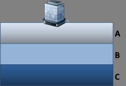
The settlement (in cm) of a structure shown in the following figure may be evaluated from
\( S=0.3A+0.2B+0.1C \)
where A, B, and C are respectively the thickness (in m) of the three layers of soil as shown. Suppose A, B, and C are modeled as independent normal random variables as
A ~ N(5,1)
B ~ N(8,2)
C ~ N(7,1)
(a) Determine the probability that the settlement will exceed 4 cm.
(b) If the total thickness of the three layers is known exactly as 20 m; and furthermore, thicknesses A and B are correlated with correlation coefficient equal to 0.5, determine the probability that the settlement will exceed 4 cm.
) \, \)
\( =1-\Phi(0.57735027)=1-0.718148613 \cong 0.282 \, \) }}
Problem 3
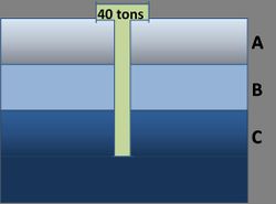
A friction pile is driven through three soil layers as shown in the following figure:
The total bearing capacity of the friction pile (in tons) is obtained from
\( Q=4A+B+2C \)
Where A, B, and C are penetration lengths (in meters) through each of the three soil layers, respectively. Suppose A ~ N(5,3); B ~ N(8,2); A and B are negatively correlated with coefficient \(\rho\) = - 0.5. The total length of the pile is 30 meters. Determine the probability that the pile will fail to support the 40 ton load, i.e., the event that the capacity Q is less than 40 tons. [Hint: Observe C = 30 - (A+B)].
) \, \)
\( =\Phi(-3.050851079) \, \)
\( \cong0.00114 \, \) }}
Problem 4
A city is located at the downstream of the confluence point of two rivers as shown. The annual maximum flood peak in River 1 has an average of \(35 m^2/sec\) with the standard deviation of \(10 m^3/sec\), whereas in River 2 the mean peak flow rate is \(25 m^3/sec\) and the standard deviation is \(10 m^3/sec\). The annual maximum peak flow rates in both rivers are normally distributed with a correlation coefficient of 0.5. Presently, the channel which runs through the city can accommodate up to \(100 m^3/sec\) flow rate without flooding the city. Please answer the following questions.
(a) What are the mean and standard deviation of the annual maximum peak discharge passing through the city?
(b) What is the annual risk that the city will experience flooding based on the existing channel capacity? What is the corresponding return period?
(c) Calculate the probability that the city will experience flooding over a 10-year period.
(d) If the desired flooding risk over a 10 year period is to be reduced by half, how large should the present channel capacity be extended to?
)=p \)
\( \Rightarrow 1-\Phi(\frac{X_0-60}{\sqrt{300}})=0.005106623 \)
\( \Rightarrow \Phi((\frac{X_0-60}{\sqrt{300}}))=0.994893377 \)
\( \Rightarrow X_0=60+\Phi^{-1}(0.994893377)\sqrt{300} \)
\( =60+2.568522177 \sqrt{300} = 104.4881091 \)
Therefore, extending the channel capacity to about \(104.5\) \(m^3/sec\) will cut the risk by half. }}
Problem 5
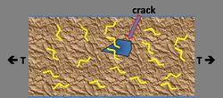
Fibers may be embedded in cement to increase its strength. Consider a cracked section as shown in the following diagram:
Suppose the total strength T of the cracked section is given by the following expression\[ T=C+(F_1+F_2+...+F_N) \]
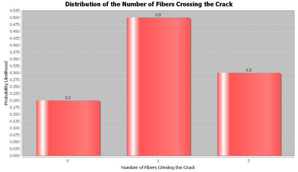
Where C is the strength contributed by the cement; \(F_1\), \(F_2\), etc. are the strength of each of the fibers across the crack; N is the total number of fibers across the crack. Suppose C=N(30,5); each \(F_i\) is N(5,3) and N is a discrete random variable with the following PMF
Assume C and \(F_i\)'s are statistically independent. What is the probability that the total strength T will be less than 30?
Problem 6
The settlement of each footing shown follows a normal distribution with a mean of 2 inches and a coefficient of variation of 30%. Suppose the settlements between two adjacent footings are correlated with a correlation coefficient of 0.7. suppose
\(D=S_1-S_2\)
where \(S_1\) and \(S_2\) are settlements of footings 1 and 2, respectively.
(a) Determine the mean and variance of D.
(b) What is the probability that the magnitude of the differential settlement (i.e., the difference between the settlements of two adjacent footings) will be less than 0.5 inch?
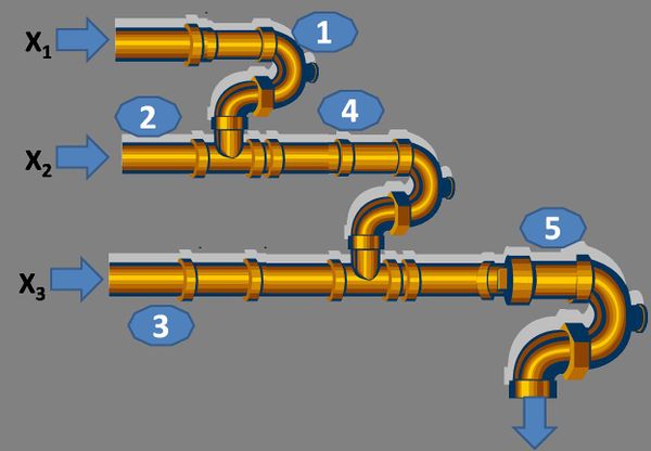
Problem 7
The systems of pipes shown in the figure is supposed to carry the storm runoffs \(X_1\) and \(X_2\), and the municipal waste water, \(X_3\). Suppose the statistics of the flow rates (all in units of cubic feet per second, CFS) are:
| Mean | c.o.v. | Distribution | |
|---|---|---|---|
| \(X_1\) | 10 | 0.3 | Normal |
| \(X_2\) | 15 | 0.2 | Normal |
| \(X_3\) | 20 | 0.00 | --- |
Because of proximity, \(X_1\) and \(X_2\) are dependent. Assume that the coefficient of correlation \(\rho_{X_1,X_2}=0.6\).
(a) Determine the mean value and standard deviation of the total rate of inflow to pipe 5.
(b) What is the probability that during a one minute interval, the volume of water flowing into pipe 2 exceeds that into pipe 1 by at least 400 cubic feet? (Hint: assume the inflow rate into each pipe is constant during that minute)
(c) Suppose the municipal waste water is projected to increase at a rate of 3 cfs per year, and pipe 5 has a capacity of 70 cfs. If the design criterion is that the probability of overflow at pipe 5 (total inflow exceeds capacity) after a storm should be less than 0.05, how many years will the current pipe 5 remain adequate, i.e., before a larger size pipe is needed?
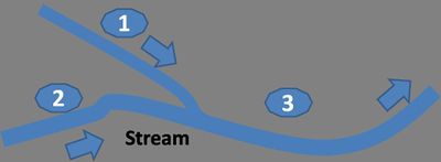
Problem 8
The flows in two tributaries 1 and 2 combine to form stream 3 as shown in the following figure:
Suppose the concentration of pollutants in tributary 1 is X which is normally distributed as N(20,4) parts per unit volume (puv); whereas that in tributary 2 is Y which is N(15,3) puv. The flow rate in tributary 1 is 600 puv cubic feet per sec (cfs) and that in 2 is 400 cfs. Hence the concentration of pollutants in the stream is
\( Z=\frac{600X+400Y}{600+400}=0.6X+0.4Y \)
Pollution occurs if pollutant concentration exceeds 20 puv.
(a) What is the probability that at least one of the two tributaries will be polluted?
(b) Assume X and Y are statistically independent. Determine the probability of a polluted stream?
(c) Suppose the same indistrial plant dumps the pollutants into the two tributaries; hence X and Y are correlated, say with \(\rho=0.8\). What is the probability of a polluted stream?
Problem 9
The actual concrete strength, Y, in a structure is generally higher than that, X, measured on specimen from the same batch of concrete. Data shows that a regression equation for predicting the actual concrete strength is
\(E(Y|x)=1.12x+0.05(ksi)\); \(0.1<x<0.5\)
and
\( Var(Y|x)=0.0025(ksi)^2 \)
Assume that Y follows a normal distribution for a given value of x.
(a) For a given job where the measured strength is 0.35 ksi, what is the probability that the actual strength will exceed the requirement of 0.3 ksi?
(b) Suppose the engineer has lost the data on the measured strength on the concrete specimen. He however recalls that is is either 0.35 or 0.40 with the relative likelihood of 1 to 4. What is the probability that the actual strength will exceed the requirement of 0.3 ksi?
(c) Suppose the measured concrete strength at two sites A and B are 0.35 and 0.4 ksi respectively. What is the probability that the actual strength for the concrete structure at site A will in fact be larger than that at site B? you may assume that the predicted actual concrete strength between sites and statistically independent.
Problem 10
A pile is designed to have a mean capacity of 20 tons; however, because of uncertainties, the pile capacity is lognormally distributed with a coefficient of variation (cov) of 20%. Suppose the pile is subject to a maximum lifetime load that is also lognormally distributed with a mean of 10 tons and a cov of 30%. Assume that pile load and capacity are statistically independent.
(a) Determine the probability of failure of the pile.
(b) A number of piles may be tied together to form a pile group to resist an external load. Suppose the capacity of the pile group is the sum of the capacities of the individual piles. Consider a pile group that consists of two single piles as described above. Because of proximity, the capacities between the two piles are correlated with a correlation coefficient of 0.8. Let T denote the capacity of this pile group.
(i) Determine the mean value and cov of T.
(ii) Will the random variable T follow a normal, or lognormal or some other probability distribution? Please substantiate.
Problem 11
A contractor submits bids to 3 highway jobs and 2 building jobs. The probability of winning each job is 0.6. The profit from a highway job is normally distributed as N(100, 40) in thousand dollars; whereas, that for a building job is N(80, 20) in thousand dollars. Assume that winning each job is an independent event and the profit between jobs are also statistically independent.
(a) What is the probability that the contractor will win at least two jobs?
(b) What is the probability that he will win exactly 1 highway job, but none of the building jobs?
(c) Suppose he has won 2 highway jobs and 1 building job. What is the probability that the total profit will exceed 300 thousand dollars?
(d) How would the answer in part (c) change if the profit form the two highway jobs are correlated with correlation coefficient ρ= 0.8?
Problem 12
During the next month, the amount of water available for a city is lognormally distributed with a mean of 1 million gallons and a c.o.v. of 40%, whereas the total demand is expected to follow a lognormal distribution with a mean of 1.5 million gallon with a c.o.v. of 10%. What is the probability of a water shortage at this city over the next month?
Problem 13
A corner column of a building is supported on a pile group consisting of 2 piles. The capacity of each pile is a sum of two independent contributions, namely the frictional resistance, F, along the pile length and the end bearing resistance, B, at the pile tip. Suppose F and B are both normally distributed with mean values of 20 and 30 tons and coefficients of variation of 0.2 and 0.3, respectively. The capacities between the two piles are correlated with a correlation coefficient of 0.8.
(a) Determine the mean and c.o.v. of the capacity of 1 pile.
(b) Determine the mean and c.o.v. of the total capacity of the pile group.
(c) If the maximum load applied to the pile group is normally distributed with a mean value of 50 tons and a c.o.v. of 0.3, what is the probability of failure of this pile group?
Problem 14
Consider a tower that is now leaning at an 18° inclination. The tower continues to lean at an annual increment A, which is normally distributed with a mean value of 0.1° and a c.o.v. of 30%.
(a) Assume that the incremental amounts of additional lean between years are statistically independent. Determine the probability that the final inclination of the tower after 16 years will exceed 20°.
(b) Suppose it is believed that the maximum inclination, M, before the tower collapses (i.e. the leaning capacity of the tower) is itself a normal random variable with a mean of 20°and a c.o.v. of 1%.
i. What is the probability that the tower will not collapse within the next 16 years?
ii. An alternative assumption (instead of statistical independence between years as in part a) is that the tower will have the same amount of incremental lean each year. What is then the probability that the tower will not collapse after 16 years?
- Back to Ebook
- SOCR Home page: http://www.socr.ucla.edu
"-----
Translate this page:

