Difference between revisions of "SOCR EduMaterials Activities ApplicationsActivities BinomialOptionPricing"
m (→Definitions) |
m (→Description) |
||
| Line 2: | Line 2: | ||
===Description=== | ===Description=== | ||
| − | You can access the | + | You can access the Binomial Option Pricing Model applet at [http://www.socr.ucla.edu/htmls/app/ the SOCR Applications Site], select ''Financial Applications'' --> ''BinomialOptionPricing''. |
===Definitions=== | ===Definitions=== | ||
Latest revision as of 15:06, 3 August 2008
Contents
[hide]SOCR Applications Activities - Binomial Option Pricing Model
Description
You can access the Binomial Option Pricing Model applet at the SOCR Applications Site, select Financial Applications --> BinomialOptionPricing.
Definitions
\[S_0\] Stock price at \(t=0\)
\[S_1\] Stock price at \(t=1\)
\[E\] Exercise price of the call option
\[u\] \(1+ \%\) change in stock price from
\[t=0\] to \(t=1\) if stock price increases (\(u>1\))
\[d\] \(1+ \%\) change in stock price from
\[t=0\] to \(t=1\) if stock price decreases (\(d<1\))
\[C\] The call price
\[\alpha\] The number of shares of stocks purchased per one call (hedge ratio)
\[C_u\] Price of call at \(t=1\) if stock price increases
\[max(S_1-E,0)\] or \(max(uS_0-E,0)\)
\[C_d\] Price of call at \(t=1\) if stock price decreases:
\[max(S_1-E,0)\] or \(max(dS_0-E,0)\)
\[r\] Continuous risk-free interest rate
- The value \(C\) of a European call option at time \(t=0\) is:
\[ C=S_0 \sum_{j=k}^{n} {n \choose j} p'^{j}(1-p')^{n-j} -
\frac{E}{e^{rt}} \sum_{j=k}^{n} {n \choose j} p^{j}(1-p)^{n-j}
\]
Where,
\[ u=e^{+\sigma \sqrt{\frac{t}{n}}}, d=e^{-\sigma \sqrt{\frac{t}{n}}}=\frac{1}{u} \]
\[ p=\frac{e^{rt}-d}{u-d}, \ \ p'=\frac{up}{e^{rt}}
\]
\[S_0\] Price of the stock at time \(t=0\)
\[E\] Exercise price at expiration
\[r\] Risk-free interest rate per period
\[n\] Number of periods
\[\sigma\] Annual standard deviation of the returns of the stock
\[t\] &Time to expiration in years
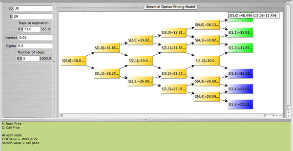
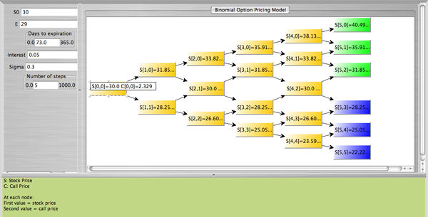
- The SOCR Binomial Option Pricing applet provides the price of the stock and the price of the call at each node. Note that at expiration the nodes for which the call is in the money (\(S > E\) are colored green, while the nodes for which the call is out of the money (\(S \le E)\) are colored blue. The example below uses the following data:
\[S_0=\$30\], \(E=\$29\), \(r_f=0.05\), \(\sigma=0.30\), \(\mbox{days to expiration}=73\), \(\mbox{number of steps}=5\).


References
The materials above was partially taken from:
- Modern Portfolio Theory by Edwin J. Elton, Martin J. Gruber, Stephen J. Brown, and William N. Goetzmann, Sixth Edition, Wiley, 2003.
- Options, Futues, and Other Derivatives by John C. Hull, Sixth Edition, Pearson Prentice Hall, 2006.
Translate this page: