SMHS TimeSeries

Scientific Methods for Health Sciences - Time Series Analysis

Overview

Time series data is a sequence of data points measured at successive pints in time spaced intervals. Time series analysis is commonly used in varieties of studies like monitoring industrial processes and tracking business metrics in the business world. In this lecture, we will present a general introduction to the time series data and introduced on some of the most commonly used techniques in the rick and rapidly growing field of time series modeling and analysis to extract meaningful statistics and other characteristics of the data. We will also illustrate the application of time series analysis techniques with examples in R.

Motivation

Economic data like daily share price, monthly sales, annual income or physical data like daily temperature, ECG readings are all examples of time series data. Time series is just an ordered sequence of values of a variable measured at equally spaced time intervals. So, what would be the effective ways to measure time series data? How can we extract information from time series data and make inference afterwards?

Theory

Time series: a sequence of data points measured at successive pints in time spaced intervals.

• Components: (1) trend component: long-run increase or decrease over time (overall upward or downward movement), typically refers to data taken over a long period of time; the trend can be upward or downward, linear or non-linear. (2) seasonal component: short-term regular wave-like patterns, usually refers to data observed within one year, which may be measured monthly or quarterly. (3) cyclical component: long-term wave-like patterns; regularly occur but may vary in length; often measured peak to peak or trough to trough. (4) irregular component: unpredictable, random, ‘residual’ fluctuation, which may be due to random variations of nature or accidents or unusual events; ‘noise’ in the time series.
• Probabilistic models: The components still add or multiply together across time.

• Simple Time Series Models:
  • Take $T_{t}$ as the trend component, $S_{t}$ as the seasonal component, $C_{t}$ as the cyclical component and $I_{t}$ as the irregular or random component. Then we have an additive model as: $x_{t}=T_{t}+S_{t}+C_{t}+I_{t};$ the multiplicative model says $x_{t}=T_{t}*S_{t}*C_{t}*I_{t};$ sometimes, we take logs on both sides of the multiplicative model to make it additive, $logx_{t}=log\left ( T_{t}*S_{t}*C_{t}*I_{t} \right )$, which can be further noted as $x_{t}{}'=T_{t}{}'+S_{t}{}'+C_{t}{}'+I_{t}{}'$.
  • Most time series models are written in terms of an (unobserved) white noise process, which is often assumed to be Gaussian: $x_{t}=w_{t}$, where $w_{t}\sim WN\left ( 0,1 \right )$, that is, $E\left ( W_{t} \right )=0, Var\left(W_{t} \right )=\sigma ^{2}$. Examples of probabilistic models include: (1) Autoregressive $x_{t}=0.6x_{t-1}+w_{t};$ (2) Moving average model $x_{t}= \frac{1}{3}\left(w_{t}+w_{t-1}+w_{t-2}\right).$
  • Fitting time series models: a time series model generates a process whose pattern can then be matched in some way to the observed data; since perfect matches are impossible, it is possible that more than one model will be appropriate for a set of data; to decide which model is appropriate: patterns suggest choices, assess within sample adequacy (diagnostics, tests), outside sample adequacy (forecast evaluation), simulation from suggested model and compare with observed data; next, turn to some theoretical aspects like how to characterize a time series, and then investigate some special processes.
  • Characterizing time series (the mean and covariance of time series): suppose the data are $x_{1},x_{2},\cdots ,x_{t},$ note for a regularly spaced time series, $x_{1}$ is observed at time $t_{0}$, $x_{2}$ is observed at $t_{0}+\Delta, x_{t}$ is observed at $t_{0}+\left( t-1\right) \Delta$; the expected value of $x_{t}$ is $\mu _{t}=E\left [ x_{t} \right ]$; the covariance function is $\gamma \left(s,t \right )=cov\left(x_{s},x_{t} \right )$. Note that, we don’t distinguish between random variables and their realizations. Properly, $x_{1},x_{2},\cdots ,x_{t}$ is a realization of some process $X_{1},X_{2},\cdots ,X_{t}$ and so $\mu _{t}=E\left [ x_{t} \right ]$ etc.
  • Characterizing time series data: weak stationarity: usually we have only one realization of the time series. There are not enough data to estimate all the means \& covariances. That is if the mean is constant, and the covariance depends only on the separation in time, then a time series is $\left(weakly\right)$ stationary. In this case $\mu_{t}=\mu$ and $\gamma\left(s,t\right)=\gamma\left(t-s\right)$. Stationary processes are much easier to handle statistically. Real time series are usually non-stationary, but can often be transformed to give a stationary process.
  • Estimation of $\gamma(h)$ (Estimating the autocovariance function): (1) for a stationary process: $\gamma(h)=\gamma(s,s+h)=cov(x_{s},x_{s+h})$ for any s.$\ \gamma (h)$ is called the autocovariance function because it measures the covariance between lags of the process $x_{t}$; (2) we observe T-h pairs separated at lag h namely $\left(x_{1},x_{h+1}\right),\cdots,\left(x_{T-h},x_{T}\right)$; the sample autocovariance function is $\hat{\gamma}(h)=\frac{1}{T}\sum_{t=1}^{T-h}\left(x_{t}-\bar{X} \right )\left(x_{t+h}-\bar{X} \right )$, note that we divide by ${T}$ although there are ${T-h}$ terms in the sum. The autocorrelation function ${ACF}$ is $\rho (h)=\frac{\gamma(h)}{\gamma(0)}$.
  • $\rho(h)$ properties: for $x_{t}$ stationary, $\gamma(h)=E(x_{t}-\mu{t})(x_{t+h}-\mu)$, where $\gamma(h)$ is an even function, that is $\gamma(h)=\gamma(-h); \left | \gamma(h) \right |\leq \left | \gamma(0) \right |$, that is $\left|\rho(h)\right|\leq1, h=\pm 1,2,\cdots$. The autocorrelation matrix, $P(h)$ is positive semi-definite which means that the autocorrelations cannot be chosen arbitrarily but must have some relations among themselves.
  • To study a set of time series data: given that we only have one realization, we need to match plot of data from proposed model with data (we can see broad/main patterns); match acf, pacf of proposed model with data (we can see if data are stationary uncorrelated, stationary autocorrelated or non-stationary); determine if the proposed model is appropriate; obtain forecasts from proposed model; compare across models that seem appropriate.
  • Large sample distribution of the $ACF$ for a $WN$ series: if $x_{t}$ is $WN$ then for n large, the sample $ACF$, $\hat{\rho}_{x}(h), h=1,2,\cdots$,H where H is fixed but arbitrary is normally distributed with zero mean and standard deviation given by $\sigma_{\hat{\rho}_{x}}(h)=\frac{1}{\sqrt{h}}$. A rule of thumb for assessing whether sample autocorrelations resemble those for a $WN$ series is by checking if approximately 95% of the sample autocorrelations are within the interval $0\pm \frac{2}{\sqrt{n}}$.
  • White noise, or stationary uncorrelated process: we say that a time series is white noise if it is weakly stationary, with $ACF$, $\rho(h)=\begin{cases} 1 & \text{ if } h=0 \\ 0 & \text{ if } h> 0\ and\ with \ E\left[w_{t} \right ]=0 \end{cases}$, i.e. white noise consists of a sequence of uncorrelated, zero mean random variables with common variance $\sigma^{2}$.

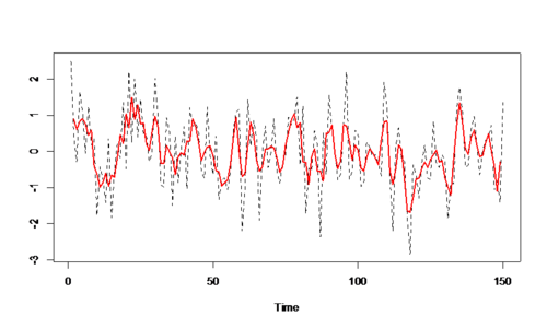
• Example of a simple moving average model in R: $v_{t}=\frac{1}{3} (w_{t-1}+w_{t}+w_{t+1})$.

R CODE: 
w <- ts(rnorm(150))  ## generate 150 data from the standard normal distribution
v <- ts(filter(w, sides=2, rep(1/3, 3)))  ## moving average model
par(mfrow=c(2,1))
plot(w,main='white noise')
plot(v,main='moving average')

or can use code:

w <- rnorm(150)  ## generate 150 data from the standard normal distribution
v <- filter(w, sides=2, rep(1/3, 3))  ## moving average model
par(mfrow=c(2,1))
plot.ts(w,main='white noise')
plot.ts(v,main='moving average')

## sums based on WN processes
ts.plot(w,v,lty=2:1,col=1:2,lwd=1:2)

The ACF and the sample ACF of some stationary processes

• white noise = $w(t),acf x(t)=w(t)+\frac{1}{3} \left(w(t-1)+w(t-2)+w(t-3) \right),$ then plot the barplot of the acf:

RCODE:
par(mfrow=c(2,1))
barplot(ARMAacf(0,lag.max=10),main='white noise=w(t)')
barplot(ARMAacf(ma=c(1/3,1/3,1/3),lag.max=10),main='acfx(t)=w(t)+1/3w(t-1)+1/3w(t-2)+1/3w(t-3)')

• Theoretical acf of some processes: Autoregressive process, $x_{t}=0.9x_{t-1}+w_{t}.$

RCODE:
par(mfrow=c(2,1))
barplot(ARMAacf(c(0.9),lag.max=30),main='acf x(t)=0.9x(t-1)+w(t)')
barplot(ARMAacf(c(1,-0.9),lag.max=30),main='acf x(t)=x(t-1)-0.9x(t-2)+w(t)')

• Recognizing patterns in probabilistic data
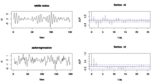
  • Example 1: compare White noise & Autoregressive process $x_{t}=w_{t} \& x_{t}=x_{t-1}-0.9x_{t-2}+w_{t})$

RCODE:
w1 <- rnorm(200)  ## generate 200 data from the standard normal distribution
x <- filter(w1, filter=c(1,-0.9),method='recursive')[-(1:50)]
w2 <- w1[-(1:50)]
xt <- ts(x)
par(mfrow=c(2,2))
plot.ts(w,main='white noise')
acf(w2,lag.max=25)
plot.ts(xt,main='autoregression')
acf(xt,lag.max=25)

• Apparently, there is almost no autocorrelation in white noise, while there is large autocorrelation in second series.

Example 2: AR & MA $x_{t}=x_{t-1}-0.9x_{t-2}+w_{t}\& v_{t}=\frac{1}{3}\left(w_{t-1}+w_{t}+w_{t+1} \right))$

RCODE:
v <- filter(w1, sides=2, rep(1/3, 3))
vt <- ts(v)[2:199]
par(mfrow=c(2,2))
plot.ts(xt,main='white noise')
acf(xt,lag.max=25)
plot.ts(vt,main='autoregression')
acf(vt,lag.max=25)

• ACF, PACF and some examples of data in R

RCODE:
data<-
c(28,22,36,26,28,28,26,24,32,30,27,24,33,21,36,32,31,25,24,25,28,36,27,32,34,30,
25,26,26,25,-
44,23,21,30,33,29,27,29,28,22,26,27,16,31,29,36,32,28,40,19,37,23,32,29,-
2,24,25,27,24,16,29,20,28,27,39,23)
par(mfrow=c(1,2))
plot(data)
qqnorm(data)
qqline(data)

data1<-data[c(-31,-55)]
par(mfrow=c(1,2))
plot.ts(data1)
qqnorm(data1)
qqline(data1)

library(astsa)
acf2(data1)

• Examining the data:

Diagnostics of outliers

RCODE:
dat<- 
c(28,22,36,26,28,28,26,24,32,30,27,24,33,21,36,32,31,25,24,25,28,36,27,32,34,30,
25,26,26,25,-44,23,21,30,    33,29,   27,29,28,22,26,27,16,31,29,36,32,28,40,19,
37,23,32,29,-2,24,25,27,24,16,29,20,28,27,  39,23)
plot.ts(dat)

Then we can easily tell that there is an outlier in this data series.

# what if we use a boxplot here?
boxplot(dat)

identify(rep(1,length(dat)),dat)   ## identify outliers by clicking on screen
## we identified the outliers are 55 and 31:
dat[31]
[1] -44
dat[55]
[1] -2
datr <- dat[c(-31,-55)]  ## this is the dat with outlier removed
qqnorm(datr)
qqline(datr)

## this plot shows that the distribution of the new data series (right) 
is closer to normal compared to the original data (left).
## The effect of outliers by comparing the ACF and PACF of the data 
series:
library(astsa)
acf2(dat)
acf2(datr)

• Diagnostics of the error: consider the model $(x_{t}=\mu+w_{t} )$ check to see if the mean of the probability distribution of error is 0; whether variance of error is constant across time; whether errors are independent and uncorrelated; whether the probability distribution of error is normal.

Residual plot for functional form

Residual plot for equal variance

Check if residuals are correlated by plotting $e_{t} vs. e_{t-1}$: there are three possible cases – positive autocorrelation, negative autocorrelation and no autocorrelation.

• Smoothing: to identify the structure by averaging out the noise since series has some structure plus variation.

Moving averages:

ma3<-filter(datr,sides=2,rep(1/3,3))
ma9<-filter(datr,sides=2,rep(1/9,9))
plot.ts(datr,ylim=c(15,50),ylab='data')
par(new=T)
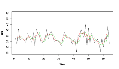
plot.ts(ma3,ylim=c(15,50),col=2,ylab='data')  ## red line indicates ma3
par(new=T)
plot.ts(ma9,ylim=c(15,50),col=3,ylab='data')  ## green line indicates ma9

• Apparently, the bigger the laggings in moving average, the smoother the time series plot of the data series.

ma3<-filter(datr,sides=2,rep(1/3,3))
ma31<-filter(datr,sides=1,rep(1/3,3))
plot.ts(datr,ylim=c(15,50),ylab='data')
par(new=T)
plot.ts(ma3,ylim=c(15,50),col=2,ylab='data')  ## red line indicates ma3
par(new=T)
plot.ts(ma31,ylim=c(15,50),col=3,ylab='data')  ## green line indicates ma31

Two sided and one sided filters with same coefficients seem to be similar in their smoothing effect.

## the effect of equal vs. unequal weights? 
ma31<-filter(datr,sides=1,rep(1/3,3))
mawt<-filter(datr,sides=1,c(1/9,1/9,7/9))
plot.ts(datr,ylim=c(15,50),ylab='data')
par(new=T)
plot.ts(ma31,ylim=c(15,50),col=2,ylab='data')  ## red line indicates ma31
par(new=T)
plot.ts(mawt,ylim=c(15,50),col=3,ylab='data')  ## green line indicates mawt

The smoothing effect of filter with equal weights seems to be bigger than the filter with unequal weights.

• Simple Exponential Smoothing (SES): premise – the most recent observations might have the highest predictive value $(\hat{x}_{t} = \alpha x_{t-1} + (1- \alpha) \hat{x}_{t-1} )$, that is new forecast = $\alpha \ actual value + (1-\alpha) \ previous forecast$. This method is appropriate for series with no trend or seasonality.

• For series with trend, can use Holt-Winters Exponential smoothing additive model $\hat{x}_{t+h}=a_{t}+h*b_{t}.$ We smooth the level or permanent component, the trend component and the seasonal component.

RCODE:
HoltWinters(series,beta=FALSE,gamma=FALSE) #simple exponential smoothing
HoltWinters(series,gamma=FALSE)  # HoltWinters trend
HoltWinters(series,seasonal= 'additive') # HoltWinters additive trend+seasonal
HoltWinters(series,seasonal= 'multiplicative') # HoltWinters multiplicative trend+seasonal

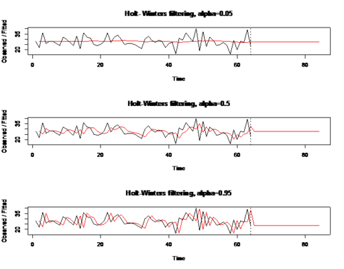
Example: RCODE: (effect of different values of alpha on datr SES)
par(mfrow=c(3,1))
exp05=HoltWinters(datr,alpha=0.05,beta=FALSE,gamma=FALSE) #simple exponential smoothing 
p05=predict(exp05,20) 
plot(exp05,p05, main = 'Holt- Winters filtering, alpha=0.05')
exp50=HoltWinters(datr, alpha=0.5,beta=FALSE,gamma=FALSE)  #simple exponential smoothing 
p50=predict(exp50,20)
plot(exp50,p50, main = 'Holt-Winters filtering, alpha=0.5')
exp95=HoltWinters(datr, alpha=0.95,beta=FALSE,gamma= FALSE)  #simple exponential smoothing 
p95=predict(exp95,20)
plot(exp95,p95,main = "Holt-Winters filtering, alpha=0.95")

• Comparing two models: we can compare ‘fit’ and forecast ability.

RCODE:
obs <- exp50$\$$x[-1]
 fit <- exp50$\$$fitted[,1]
r1 <- obs-fit
plot(r1)
par(mfrow=c(1,2))
plot(r1)
acf(r1)

• Regression based (nonparametric) smoothing: (1) kernel: extension of a two-sided MA. Use a bandwidth (number of terms) plus a kernel function to smooth a set of values, ksmooth; (2) local linear regression (loess): fit local polynomial regression and join them together, loess; (3) fitting cubic splines: extension of polynomial regression, partition data and fit separate piecewise regression to each section, smooth them together where they join, smooth.spine; (4) many more, lowess, supsmu.

•Kernel smoother: define bandwidth; choose a kernel; use robust regression to get smooth estimate; bigger the bandwidth, smoother the result

•Loess: define the window width; choose a weight function; use polynomial regression and weighted least squares to get smoothest estimate; the bigger span, the smoother the result.

•Splines: divide data into intervals; in each interval, fit a polynomial regression of order p such that the splines are continuous at knots; use a parameter (spar in R) to smooth the splines; the bigger the spar, the smoother the result.

•Issues with regression based (nonparametric) smoothing: (1) the size of S has an important effect on the curve; (2) a span that is too small (meaning that insufficient data fall within the window) produces a curve characterized by a lot of noise, results in a large variance; (3) if the span is too large, the regression will be oversmoothed, and thus the local polynomial may not fit the data well. This may result in loss of important information, and thus the fit will have large bias; (4) we want the smallest span that provides a smooth structure.

• A regression model for trend: given $y_{t}, t=1,2,…,\cdots,$ T is a time series, fit a regression model for trend. The plot suggests that we fit a trend line, say $y_{t}=\beta_{1}+\beta_{2} t + \varepsilon_{t}$.

•Assumptions: variance of error is constant across observations; errors are independent / uncorrelated across observations; the regressor variables and error are independent; we may also assume probability distribution of error is normal.

RCODE
fit <- lm(x~z)
summary(fit$\$$coeff)
 plot.ts(fit$\$$resid)  # plot the residuals of the fitted regression model
acf2(fit$\$$resid)  # the ACF and PACF of the residuals of the fitted regression model
 qqnorm(fit$\$$resid)
qqline(fit$\$$resid)
 

*Analyzing patterns in data and modeling: seasonality
**Exploratory analysis

 RCODE:
 data=c( 118,132,129,121,135,148,148,136,119,104,118,115,126,141,135,125,
 149,170,170,158,133,114,140,145,150,178,163,172,178,199,199,184,162,146,
 166,171,180,193,181,183,218,230,242,209,191,172,194,196,196,236,235,
 229,243,264,272,237,211,180,201,204,188,235,227,234,264,302,293,259,229,
 203,229,242,233,267,269,270,315,364,347,312,274,237,278,284,277,317,313,
 318,374,413,405,255,306,271,306,300)
 air <- ts(data,start=c(1949,1),frequency=12)
 y <- log(air)
 par(mfrow=c(1,2))
 plot(air)
 plot(y)


[[Image:SMHS_Fig21_TimeSeries.png|500px]]


 ## from the charts above, taking log helps a little bit with the increasing variability. 

 monthplot(y)


[[Image:SMHS_Fig22_TimeSeries.png|500px]]


 acf2(y)

[[Image:SMHS_Fig23_TimeSeries.png|500px]]

*Smoothing: the Holt-Winters method smooths and obtains three parts of a series: level, trend and seasonal. The method requires smoothing constants: your choice or those which minimize the one step ahead forecast error: $\sum_{t=1}^{T} \left(\hat{x}_{t} - x_{t-1} \right )^{2}$, where $t=1,2,\cdots,T$. So at a given time point, smoothed value = (level+h*trend)+seasonal index (additive); data value = (level+h*trend)*seasonal index (multiplicative). Additive: $\hat{x}_{t+h}=a_{t}+h*b_{t}+s_{t+1+(h-1)\mod{p}}$; Multiplicative: $\hat{x}_{t+h}=(a_{t}+h*b_{t})* s_{t+1+(h-1)\mod{p}}.$


 RCODE:
 par(mfrow=c(2,1))
 sa <- HoltWinters(air,seasonal=c('additive'))
 psa <- predict(sa,60)
 plot(sa,psa,main='Holt-Winters filtering, airline passengers, HW additive')
 sm <- HoltWinters(air,seasonal=c('multiplicative'))
 psam <- predict(sm,60)
 plot(sm,psam,main='Holt-Winters filtering, airline passengers, HW multiplicative')

[[Image:SMHS_Fig24_TimeSeries.png|500px]]

## seasonal decomposition using loess, log(airpassengers)

[[Image:SMHS_Fig25_TimeSeries.png|500px]]

*Regression: estimation, diagnostics, interpretation. Defining dummy variables to capture the seasonal effect in regression. If there is a variable with k categories, there will be k-1 dummies if the intercept is included in the regression (exclude one group); there will be k dummies if the intercept is not included in the regression; if the intercept is included in the regression, the coefficient of a dummy variable is always the difference of means between that group and the excluded group. 

 RCODE:
 t <- time(y)
 Q <- factor(rep(1:12,8))
 h <- lm(y~time(y)+Q)  # regression with intercept, drops first category = January
 model.matrix(h)
 h1 <- lm(y~0+time(y)+Q)  # regression without intercept
 model.matrix(h1)
 x1 <- ts(y[1:72],start=c(1949,1),frequency=12)
 t1 <- t[1:72]
 Q1 <- Q[1:72]
 contrasts(Q1)=contr.treatment(12,base=10)
 h2 <- lm(x1~t1+Q1)  # regression with intercept, drops 10th category = October
 model.matrix(h2)
 reg <- lm(x1~t1+Q1)
 par(mfrow=c(2,2))
 plot.ts(reg$\$$resid)
qqnorm(reg$\$$resid)
 qqline(reg$\$$resid)
acf(reg$\$$resid)
 pacf(reg$\$$resid)

## forecasts RCODE
newdata=data.frame(t1=t[73:96], Q1=Q[73:96]) 
preg=predict(reg,newdata,se.fit=TRUE) 
seup=preg$\$$fit+2*preg$\$$se.fit
seup 
       1        2        3        4        5        6        7        8        9 
5.577144 5.722867 5.679936 5.667979 5.780376 5.881420 5.889829 5.782526 5.655445 
      10       11       12       13       14       15       16       17       18 
5.525933 5.661158 5.681042 5.716577 5.862300 5.819369 5.807412 5.919809 6.020853 
      19       20       21       22       23       24 
6.029262 5.921959 5.794878 5.665366 5.800591 5.820475 
selow=preg$\$$fit-2*preg$\$$se.fit
selow
       1        2        3        4        5        6        7        8        9 
5.479442 5.625165 5.582234 5.570277 5.682674 5.783718 5.792127 5.684824 5.557743 
      10       11       12       13       14       15       16       17       18 
5.428232 5.563456 5.583340 5.610927 5.756650 5.713720 5.701763 5.814160 5.915203 
      19       20       21       22       23       24 
5.923613 5.816309 5.689228 5.559717 5.694941 5.714825

x1r=y[73:96]
t1r=t[73:96]
plot(t1r,x1r, col='red',lwd=1:2,main='Actual vs Forecast', type='l')
lines(t1r,preg$\$$fit, col='green', lwd=1:2)
 lines(t1r,seup, col='blue', lwd=1:2)
 lines(t1r,selow, col='blue', lwd=1:2)
 ## red refer actual; green refers to forecast; blue refers to standard error

[[Image:SMHS_Fig27_TimeSeries.png|500px]]

 ## Holt Winters smoothing: forecasts
 sa=HoltWinters(x1, seasonal = c("additive"))
 psa=predict(sa,24)
 plot(t1r,x1r, col="red",type="l",main = "Holt- Winters filtering, airline passengers, HW additive")
 lines(t1r, psa, ,col="green")

 ## red represents the actual, green: forecast

[[Image:SMHS_Fig28_TimeSeries.png|500px]]

 sqrt(sum(x1r-psa)^2)) ##HW
 [1] 0.3988259
 sqrt(sum((x1r-preg$\$$fit)^2)) ##reg
[1] 0.3807665

## not sure about the mod here?!

RCODE:
par(mfrow=c(2,1))
sa <- HoltWinters(air,seasonal=c('additive'))
psa <- predict(sa,60)
plot(sa,psa,main='Holt-Winters filtering, airline passengers, HW additive')
sm <- HoltWinters(air,seasonal=c('multiplicative'))
psam <- predict(sm,60)
plot(sm,psam,main='Holt-Winters filtering, airline passengers, HW multiplicative')

1. 1. seasonal decomposition using loess, log(airpassengers)

• Regression: estimation, diagnostics, interpretation. Defining dummy variables to capture the seasonal effect in regression. If there is a variable with k categories, there will be k-1 dummies if the intercept is included in the regression (exclude one group); there will be k dummies if the intercept is not included in the regression; if the intercept is included in the regression, the coefficient of a dummy variable is always the difference of means between that group and the excluded group.

RCODE:
$t <- time(y)$
$Q <- factor(rep(1:12,8))$
$h <- lm(y~time(y)+Q)$  # regression with intercept, drops first category = January
model.matrix(h)
$h1 <- lm(y~0+time(y)+Q)$  # regression without intercept
model.matrix(h1)
$x1 <- ts(y[1:72]$,start=c(1949,1),frequency=12)
t1 <- t[1:72]
Q1 <- Q[1:72]
contrasts(Q1)=contr.treatment(12,base=10)
h2 <- lm(x1~t1+Q1)  # regression with intercept, drops 10th category = October
model.matrix(h2)
reg <- lm(x1~t1+Q1)
par(mfrow=c(2,2))
plot.ts(reg$resid)
qqnorm(reg$resid)
qqline(reg$resid)
acf(reg$resid)
pacf(reg$resid)

## forecasts RCODE
newdata=data.frame(t1=t[73:96], Q1=Q[73:96])
preg=predict(reg,newdata,se.fit=TRUE) 
seup=preg$fit+2*preg$se.fit
seup

Applications

1)This article presents a comprehensive introduction to the filed of time series analysis. It discussed about the common patterns existing in time series data and introduced some commonly used techniques to deal with time series data and ways to analyze time series.

2)This article investigates whether macroeconomic time series are better characterized as stationary fluctuations around a deterministic trend or as non-stationary processes that have no tendency to return to a deterministic path. Using long historical time series for the U.S. we are unable to reject the hypothesis that these series are non-stationary stochastic processes with no tendency to return to a trend line. Based on these findings and an unobserved components model for output that decomposes fluctuations into a secular or growth component and a cyclical component we infer that shocks to the former, which we associate with real disturbances, contribute substantially to the variation in observed output. We conclude that macroeconomic models that focus on monetary disturbances as a source of purely transitory fluctuations may never be successful in explaining a large fraction of output variation and that stochastic variation due to real factors is an essential element of any model of macroeconomic fluctuations.

Software

See the CODE examples given in this lecture.

Problems

1) Consider a signal-plus-noise model of the general form x_{t}=s_{t}+w_{t}, where w_{t} is Gaussian white noise with \sigma ^{2} _{w} = 1. Simulate and plot n=200 observations from each of the following two models. (a) x_{t} = s_{t}+w_{t}, for t=1,2,\cdots,200, where s_{t}=\begin{cases} 0 & \text{ if } t=1,2,cdots,100 \\ & 10exp \left \{ -(t-100)/20) \right \} cos\left ( 2\pi t/4 \right )\text{ if } t=101,102,\cdots,200 \end{cases} . (b) x_{t}=s_{t}+w_{t}, for t=1,2,\cdots, 200, where s_{t}=\begin{cases} 0 & \text{ if } t=1,2,cdots,100 \\ & 10exp \left \{ -(t-100)/200) \right \} cos\left ( 2\pi t/4 \right )\text{ if } t=101,102,\cdots,200 \end{cases}. (c) Compare the signal modulators (a) exp \left \{-t/20 \right \} and (b) exp \left \{-t/200 \right \}, for t=1,2, cdots,100.

2) (a) Generate n=100 observations from the autoregression x_{t}=-0.9 x_{t-2} +w_{t}, with \signma {w}=1, using the method described in Example 1.10, page 13 given in the textbook. Next, apply the moving average filter v_{t}=\left(x_{t}+x_{t-1}+x_{t-2}+x_{t-3} \right )/4 to x_{t}, the data you generated. Now, plot x_{t} as a line and superimpose v_{t} as a dashed line. Comment on the behavior of x_{t} and how apply the moving average filter changes that behavior. [Hint: use v=filter(x,rep(1/4,4),sides=1) for the filter]. (b) Repeat (a) but with x_{t}=cos \left( 2 \pi t/4 \right). (c) Repeat (b) but with added N(0,1) noise, x_{t}=cos \left(2 \pi t/4 \right) +w_{t}. (d) Compare and contrast (a) – (c).

3) For the two series, x_{t} in 6.1 (a) and (b): (a) Compute and plot the mean functions \mu _{x} (t) for t=1,2,\cdots,200. (b) Calculate the autocovariance functions, \gamma _{x} (s,t), for s,t=1,2, \cdots, 200.

4) Consider the time series x_{t} = \beta {1} + \beta {2} t + w{t}, where \beta _{1} and \beta_{2} are known constants and w_{t} is a white noise process with variance \sigma ^{2} _{w}. (a) Determine whether x_{t} is stationary. (b) Show that the process y_{t}=x_{t} – x_{t-1} is stationary. (c) Show that the mean of the moving average v_{t}= \frac {1}{2q+1} \sum_{j=-q}^{q} x_{t-j}, is \beta _{1} + \beta _{2} t, and give a simplified expression for the autocovariance function.

---

• SOCR Home page: http://www.socr.umich.edu

---

---

Translate this page:

(default)	Deutsch	Español	Français	Italiano	Português	日本語	България	الامارات العربية المتحدة	Suomi	इस भाषा में	Norge
한국어	中文	繁体中文	Русский	Nederlands	Ελληνικά	Hrvatska	Česká republika	Danmark	Polska	România	Sverige