Difference between revisions of "AP Statistics Curriculum 2007 Laplace"
(→Related Distributions) |
(→Applications) |
||
| Line 49: | Line 49: | ||
*Insurance claims | *Insurance claims | ||
*Structural changes in switching-regime model and Kalman filter | *Structural changes in switching-regime model and Kalman filter | ||
| + | |||
| + | ===Example=== | ||
| + | Suppose that the return of a certain stock has a Laplace distribution with <font size=3><math>\mu=5</math></font> and <font size=3><math>b=2</math></font>. Compute the probability that the stock will have a return between 6 and 10. | ||
| + | |||
| + | We can compute this as follows: | ||
| + | |||
| + | :<math>P(6 \le X\le 10)=\sum_{x=6}^{10}\frac{1}{2\times 2}\exp(-\frac{|x-5|}{2})=0.262223</math> | ||
| + | |||
| + | The figure below shows this result using [http://socr.ucla.edu/htmls/dist/Laplace_Distribution.html SOCR distributions] | ||
| + | <center>[[Image:Laplace.jpg|600px]]</center> | ||
Revision as of 16:13, 11 July 2011
Laplace Distribution
Definition: Laplace distribution is a distribution that is symmetrical and more “peaky” than a normal distribution. The dispersion of the data around the mean is higher than that of a normal distribution. Laplace distribution is also sometimes called the double exponential distribution.
Probability density function: For X~Laplace(\(\mu\),b), the Laplace probability density function is given by
\[\frac{1}{2b}exp(-\frac{|x-\mu|}{b})\]
where
- e is the natural number (e = 2.71828…)
- b is a scale parameter (determines the profile of the distribution)
- \(\mu\) is the mean
- x is a random variable
Cumulative density function: The Laplace cumulative distribution function is given by
\[ \left\{\begin{matrix} \frac{1}{2}\exp(\frac{x-\mu}{b}) & \mbox{if }x < \mu \\[8pt] 1-\frac{1}{2}\exp(-\frac{x-\mu}{b}) & \mbox{if }x \geq \mu \end{matrix}\right. \]
where
- e is the natural number (e = 2.71828…)
- b is a scale parameter (determines the profile of the distribution)
- \(\mu\) is the mean
- x is a random variable
Moment generating function: The Laplace moment-generating function is
\[M(t)=\frac{\exp(\mu t)}{1-b^2 t^2} \mbox{ for }|t|<\frac{1}{b}\]
Expectation:
\[E(X)=\mu\!\]
Variance: The gamma variance is
\[Var(X)=2b^2\!\]
Related Distributions
- If \(X\sim Laplace(\mu,b)\!\), then \(kX+b\sim Laplace(k\mu+b,kb)\!\)
- If \(X \sim Laplace(0,b)\!\), then \(|X| \sim Exponential(\tfrac{1}{b})\!\) (exponential distribution)
Applications
The Laplace distribution is used for modeling in signal processing, various biological processes, finance, and economics. Examples of events that may be modeled by Laplace distribution include:
- Credit risk and exotic options in financial engineering
- Insurance claims
- Structural changes in switching-regime model and Kalman filter
Example
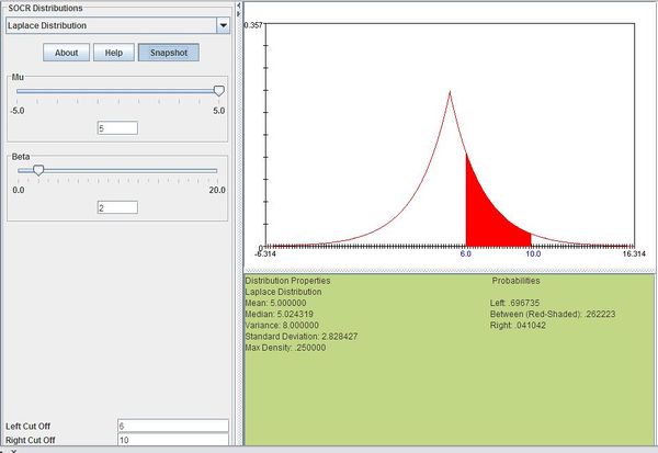
Suppose that the return of a certain stock has a Laplace distribution with \(\mu=5\) and \(b=2\). Compute the probability that the stock will have a return between 6 and 10.
We can compute this as follows:
\[P(6 \le X\le 10)=\sum_{x=6}^{10}\frac{1}{2\times 2}\exp(-\frac{|x-5|}{2})=0.262223\]
The figure below shows this result using SOCR distributions
