Difference between revisions of "SMHS LinearModeling"
(Created page with "== Scientific Methods for Health Sciences - Linear Modeling == ===Statistical Software- Pros/Cons Comparison=== Using the SOCR_Simulated_HELP_Data|SOCR Health Eval...") |
|||
| Line 2: | Line 2: | ||
===Statistical Software- Pros/Cons Comparison=== | ===Statistical Software- Pros/Cons Comparison=== | ||
| − | |||
| − | + | ===Quality Control=== | |
| − | # | + | '''Questions: |
| − | + | *''' Is the data what it’s supposed to (does it represent the study cohort/population)? | |
| + | *''' How to inspect the quality of the data? | ||
| + | |||
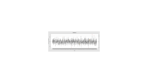
| + | Data Quality Control (QC) and Quality Assurance (QA) represent important components of all modeling, analytics and visualization that precede all subsequent data processing steps. QC and QA may be performed manually or automatically. Statistical quality control involves quantitative methods for monitoring and controlling a process or data derived from observing a natural phenomenon. For example, is there evidence in the plots below of a change in the mean of these processes? | ||
| + | |||
| + | # simulate data with base value of 100 w/ normally distributed error | ||
| + | # install.packages("qcc") | ||
| + | library(qcc) | ||
| + | demo.data.1 <- rep(100, 1000) + rnorm(1000, mean=0, sd=2) | ||
| + | qcc(demo.data.1, type="xbar.one", center=100, add.stats=FALSE, | ||
| + | title="Simulation 1", xlab="Index") | ||
| + | |||
| + | [[Image:SMHS_LinearModeling_Fig1.png|500px]] | ||
| + | |||
attach(data_1) | attach(data_1) | ||
Revision as of 08:33, 21 January 2016
Scientific Methods for Health Sciences - Linear Modeling
Statistical Software- Pros/Cons Comparison
Quality Control
Questions:
- Is the data what it’s supposed to (does it represent the study cohort/population)?
- How to inspect the quality of the data?
Data Quality Control (QC) and Quality Assurance (QA) represent important components of all modeling, analytics and visualization that precede all subsequent data processing steps. QC and QA may be performed manually or automatically. Statistical quality control involves quantitative methods for monitoring and controlling a process or data derived from observing a natural phenomenon. For example, is there evidence in the plots below of a change in the mean of these processes?
# simulate data with base value of 100 w/ normally distributed error
# install.packages("qcc")
library(qcc)
demo.data.1 <- rep(100, 1000) + rnorm(1000, mean=0, sd=2)
qcc(demo.data.1, type="xbar.one", center=100, add.stats=FALSE,
   title="Simulation 1", xlab="Index")
attach(data_1)
# to ensure all variables are accessible within R, e.g., using age instead of data_1$\$$age
 # i2 maximum number of drinks (standard units) consumed per day (in the past 30 days range 0–184) see also i1
 # treat randomization group (0=usual care, 1=HELP clinic)
 # pcs SF-36 Physical Component Score (range 14-75)
 # mcs SF-36 Mental Component Score(range 7-62)
 # cesd Center for Epidemiologic Studies Depression scale (range 0–60)
 # indtot Inventory of Drug Use Con-sequences (InDUC) total score (range 4–45)
 # pss_fr perceived social supports (friends, range 0–14) see also dayslink
 # drugrisk Risk-Assessment Battery(RAB) drug risk score (range0–21)
 # satreat any BSAS substance abuse treatment at baseline (0=no,1=yes)

==='"`UNIQ--h-3--QINU`"'Fragment of the data===
<center>
{| class="wikitable" style="text-align:center; " border="1"
|-
! ID ||i2 ||age ||treat ||homeless ||pcs ||mcs ||cesd ||indtot ||pss_fr ||drugrisk ||sexrisk ||satreat ||female ||substance ||racegrp
|-
| 1 ||0 ||25 ||0 ||0 ||49 ||7 ||46 ||37 ||0 ||1 ||6 ||0 ||0 ||cocaine ||black
|-
| 2 ||18 ||31 ||0 ||0 ||48 ||34 ||17 ||48 ||0 ||0 ||11 ||0 ||0 ||alcohol ||white
|-
| 3 ||39 ||36 ||0 ||0 ||76 ||9 ||33 ||41 ||12 ||19 ||4 ||0 ||0 ||heroin ||black
|-
| … || || || || || || || || || || || || || || ||
|-
| 100 ||81 ||22 ||0 ||0 ||37 ||17 ||19 ||30 ||3 ||0 ||10 ||0 ||0 ||alcohol ||other
|}
</center>

==='"`UNIQ--h-4--QINU`"'Testing section===

 summary(data_1)

 x.norm <- rnorm(n=200, m=10, sd=20)
 hist(x.norm, main="N(10,20) Histogram")
 hist(x.norm, main="N(10,20) Histogram")
 mean(data_1$\$$age)
sd(data_1$\$$age)
Simulate new data to match the properties/characteristics of observed data
- i2 [0: 184]
- age m=34,sd=12
- treat {0,1}
- homeless {0,1}
- pcs 14-75
- mcs 7-62
- cesd 0–60
- indtot 4-45
- pss_fr 0-14
- drugrisk 0-21
- sexrisk
- satreat (0=no,1=yes)
- female (0=no,1=yes)
- racegrp (black, white, other)
# Demographics variables
Sex <- ifelse(runif(NumSubj)<.5,0,1)
Weight <- as.integer(rnorm(NumSubj, 80,10))
Age <- as.integer(rnorm(NumSubj, 62,10))
# Diagnosis:
Dx <- c(rep("PD", 100), rep("HC", 100), rep("SWEDD", 82))
# Genetics
chr12_rs34637584_GT <- c(ifelse(runif(100)<.3,0,1), ifelse(runif(100)<.6,0,1), ifelse(runif(82)<.4,0,1))                              # NumSubj Bernoulli trials
chr17_rs11868035_GT <- c(ifelse(runif(100)<.7,0,1), ifelse(runif(100)<.4,0,1), ifelse(runif(82)<.5,0,1))                              # NumSubj Bernoulli trials
# Clinical          # rpois(NumSubj, 15) + rpois(NumSubj, 6)
UPDRS_part_I <- c( ifelse(runif(100)<.7,0,1)+ifelse(runif(100)<.7,0,1),
ifelse(runif(100)<.6,0,1)+ ifelse(runif(100)<.6,0,1),
ifelse(runif(82)<.4,0,1)+ ifelse(runif(82)<.4,0,1) )
UPDRS_part_II <- c(sample.int(20, 100, replace=T), sample.int(14, 100, replace=T),
sample.int(18, 82, replace=T) )
UPDRS_part_III <- c(sample.int(30, 100, replace=T), sample.int(20, 100, replace=T),
   sample.int(25, 82, replace=T) )
# Time: VisitTime – done automatically below in aggregator
# Data (putting all components together)
sim_PD_Data <- cbind(
          rep(Cases, each= NumTime),                          # Cases
          rep(L_caudate_ComputeArea, each= NumTime), # Imaging
          rep(Sex, each= NumTime),                            # Demographics
          rep(Weight, each= NumTime),
          rep(Age, each= NumTime),
          rep(Dx, each= NumTime),                             # Dx
          rep(chr12_rs34637584_GT, each= NumTime),            # Genetics
          rep(chr17_rs11868035_GT, each= NumTime),
          rep(UPDRS_part_I, each= NumTime),                   # Clinical
          rep(UPDRS_part_II, each= NumTime),
          rep(UPDRS_part_III, each= NumTime),
          rep(c(0,6,12,18), NumSubj)                          # Time
)
# Assign the column names
colnames(sim_PD_Data) <- c(
"Cases",
"L_caudate_ComputeArea",
"Sex", "Weight", "Age",
"Dx", "chr12_rs34637584_GT", "chr17_rs11868035_GT",
"UPDRS_part_I", "UPDRS_part_II", "UPDRS_part_III",
"Time"
)
# some QC
summary(sim_PD_Data)
dim(sim_PD_Data)
head(sim_PD_Data)
.....

....
- SOCR Home page: http://www.socr.umich.edu
Translate this page:
