SMHS BigDataBigSci CrossVal

Questions

• What does it mean to validate a result, a method, approach, protocol, or data?

• Can we do “pretend” validations that closely mimic reality?

Validation is the scientific process of determining the degree of accuracy of a mathematical, analytic or computational model as a representation of the real world based on the intended model use. There are various challenges with using observed experimental data for model validation:

1. Incomplete details of the experimental conditions may be subject to boundary and initial conditions, sample or material properties, geometry or topology of the system/process.

2. Limited information about measurement errors due to lack of experimental uncertainty estimates.

Empirically observed data may be used to evaluate models with conventional statistical tests applied subsequently to test null hypotheses (e.g., that the model output is correct). In this process, the discrepancy between some model-predicted values and their corresponding/observed counterparts are compared. For example, a regression model predicted values may be compared to empirical observations. Under parametric assumptions of normal residuals and linearity, we could test null hypotheses like slope = 1 or intercept = 0. When comparing the model obtained on one training dataset to an independent dataset, the slope may be different from 1 and/or the intercept may be different from 0. The purpose of the regression comparison is a formal test of the hypothesis (e.g., slope = 1, mean _observed =mean_predicted, then the distributional properties of the adjusted estimates are critical in making an accurate inference. The logistic regression test is another example for comparing predicted and observed values. Measurement errors may creep in, due to sampling or analytical biases, instrument reading or recording errors, temporal or spatial sampling sample collection discrepancies, etc.

Cross-validation

Cross-validation is a method for validating of models by assessing the reliability and stability of the results of a statistical analysis (e.g., model predictions) based on independent datasets. For prediction of trend, association, clustering, etc., a model is usually trained on one dataset (training data) and tested on new unknown data (testing dataset). The cross-validation method defines a test dataset to evaluate the model avoiding overfitting (the process when a computational model describes random error, or noise, instead of underlying relationships in the data).

Overfitting

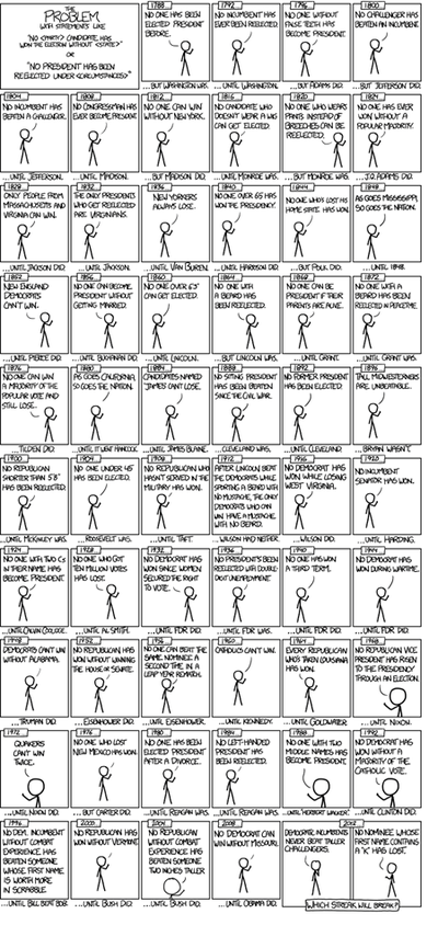
Example (US Presidential Elections): By 2014, there have been only 56 presidential elections and 43 presidents. That is a small dataset, and learning from it may be challenging. If the predictor space expands to include things like having false teeth, it's pretty easy for the model to go from fitting the generalizable features of the data (the signal) and to start matching the noise. When this happens, the quality of the fit on the historical data may improve (e.g., better R²), but the model may fail miserably when used to make inferences about future presidential elections.

(Figure from http://xkcd.com/1122/)

Example (Google Flu Trends): A March 14, 2014 article in Science (DOI: 10.1126/science.1248506), identified problems in Google Flu Trends (http://www.google.org/flutrends/about/#US), DOI 10.1371/journal.pone.0023610, which may be attributed in part to overfitting. In February 2013, Nature reported that GFT was predicting more than double the proportion of doctor visits for influenza-like illness (ILI) than the Centers for Disease Control and Prevention (CDC), despite the fact that GFT was built to predict CDC reports.

GFT model found the best matches among 50 million search terms to fit 1,152 data points. The odds of finding search terms that match the propensity of the flu but are structurally unrelated, and so do not predict the future, were quite high. GFT developers, in fact, report weeding out seasonal search terms unrelated to the flu but strongly correlated to the CDC data, e.g., high school basketball season. The big GFT data may have overfitted the small number of cases. The GFT approach missed the non-seasonal 2009 influenza A–H1N1 pandemic.

Example (Autism). Autistic brains constantly overfit visual and cognitive stimuli. To an autistic person, a general conversation of several adults may seem like a cacophony due to super-sensitive detail-oriented hearing and perception tuned to literally pick up all elements of the conversation and the environment but downplay body language, sarcasm and non-literal cues. We can miss the forest for the trees when we start "overfitting," over-interpreting the noise on top of the actual signal. Ambient noise, trivial observations and unrelated perceptions may hide the true communication details.

During each communication (conversation) there are exchanges of both information and random noise. Fitting a perfect model is only listening to the “relevant” information. Over-fitting is when your attention is (excessively) consumed with the noise, or worse, letting the noise drown out the information exchange.

Any dataset is a mix of signal and noise. The main task of our brains are to sort these components and interpret the information (i.e., ignore the noise).

Our predictions are most accurate if we can model as much of the signal as possible and as little of the noise as possible. Note that in these terms, R² is a poor metric to identify predictive power - it measures how much of the signal and the noise is explained by our model. In practice, it's hard to always identify what's signal and what's noise. This is why practical applications tends to favor simpler models, since the more complicated a model is the easier it is to overfit the noise component in the information.

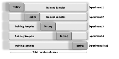
Cross-validation is an iterative process, where each step involves:

• Randomly partitioning a sample of data into 2 complementary subsets (training + testing),

• Performing the analysis on the training subset,

• Validating the analysis on the testing subset

• Increase the iteration index and repeat the process (termination criterial can involve a fixed number, or a desired (mean?) variability or error-rate.

The validation results at each iteration are averaged, to reduce noise/variability, and reported.

Cross-validation guards against testing hypotheses suggested by the data themselves (aka as "Type III errors", False-Suggestion) in cases when new observations are hard to obtain (due to costs, reliability, time or other constraints).

Cross-validation is different from conventional-validation (e.g. 80%-20% partitioning the data set into training and testing subsets) as the in the conventional validation, the error (e.g. Root Mean Square Error, RMSE) on the training data is not a useful estimator of model performance, as it does not generalize across multiple samples. Errors of the conventional-valuation based on the results on the test data do not assess model performance, in general. A more fair way to properly estimate model prediction performance is to use cross-validation, which combines (averages) prediction errors or measures of fit to correct for the stochastic nature of training and testing data partitions and generate a more accurate and robust estimate of real model performance.

A more complex model overfits-the-data, relative to a simpler model when the former generates accurate fitting results for known data but less accurate results when predicting based on new data (foresight). Knowledge from past experience includes information either relevant or irrelevant (noise) for the future information. In challenging data-driven predict models when uncertainty (entropy) is high, more noise is present in past information that needs to be ignored in future forecasting. However it is generally hard to discriminate patterns from noise in complex systems (i.e., deciding which part to model and which to ignore). Models that reduce the chance of fitting noise are called robust.

Example (Linear Regression)

We can demonstrate model assessment using linear regression. Suppose we observe response values {y₁,...,y_n }, and the corresponding k predictors represented as a kD vector of covariates {x₁,...,x_n }, where subjects/cases are indexed by 1 ≤ i ≤ n, and the data-elements (variables) are indexed by 1 ≤ j ≤ k.

See also

• Structural Equation Modeling (SEM)
• Growth Curve Modeling (GCM)
• Generalized Estimating Equation (GEE) Modeling
• Back to Big Data Science

---

• SOCR Home page: http://www.socr.umich.edu

---

---

Translate this page:

(default)	Deutsch	Español	Français	Italiano	Português	日本語	България	الامارات العربية المتحدة	Suomi	इस भाषा में	Norge
한국어	中文	繁体中文	Русский	Nederlands	Ελληνικά	Hrvatska	Česká republika	Danmark	Polska	România	Sverige