SMHS BigDataBigSci CrossVal

Big Data Science - (Internal) Statistical Cross-Validaiton

Questions

What does it mean to validate a result, a method, approach, protocol, or data?
Can we do “pretend” validations that closely mimic reality?

Validation is the scientific process of determining the degree of accuracy of a mathematical, analytic or computational model as a representation of the real world based on the intended model use. There are various challenges with using observed experimental data for model validation:

1. Incomplete details of the experimental conditions may be subject to boundary and initial conditions, sample or material properties, geometry or topology of the system/process.

2. Limited information about measurement errors due to lack of experimental uncertainty estimates.

Empirically observed data may be used to evaluate models with conventional statistical tests applied subsequently to test null hypotheses (e.g., that the model output is correct). In this process, the discrepancy between some model-predicted values and their corresponding/observed counterparts are compared. For example, a regression model predicted values may be compared to empirical observations. Under parametric assumptions of normal residuals and linearity, we could test null hypotheses like slope = 1 or intercept = 0. When comparing the model obtained on one training dataset to an independent dataset, the slope may be different from 1 and/or the intercept may be different from 0. The purpose of the regression comparison is a formal test of the hypothesis (e.g., slope = 1, mean _observed =mean_predicted, then the distributional properties of the adjusted estimates are critical in making an accurate inference. The logistic regression test is another example for comparing predicted and observed values. Measurement errors may creep in, due to sampling or analytical biases, instrument reading or recording errors, temporal or spatial sampling sample collection discrepancies, etc.

Overview

Cross-validation

Cross-validation is a method for validating of models by assessing the reliability and stability of the results of a statistical analysis (e.g., model predictions) based on independent datasets. For prediction of trend, association, clustering, etc., a model is usually trained on one dataset (training data) and tested on new unknown data (testing dataset). The cross-validation method defines a test dataset to evaluate the model avoiding overfitting (the process when a computational model describes random error, or noise, instead of underlying relationships in the data).

Overfitting

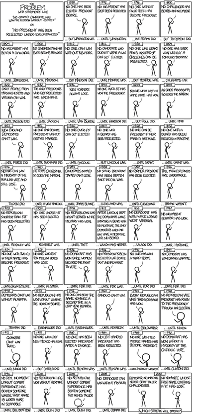
Example (US Presidential Elections): By 2014, there have been only 56 presidential elections and 43 presidents. That is a small dataset, and learning from it may be challenging. If the predictor space expands to include things like having false teeth, it's pretty easy for the model to go from fitting the generalizable features of the data (the signal) and to start matching the noise. When this happens, the quality of the fit on the historical data may improve (e.g., better R²), but the model may fail miserably when used to make inferences about future presidential elections.

(Figure from http://xkcd.com/1122/)

Example (Google Flu Trends): A March 14, 2014 article in Science (DOI: 10.1126/science.1248506), identified problems in Google Flu Trends (http://www.google.org/flutrends/about/#US), DOI 10.1371/journal.pone.0023610, which may be attributed in part to overfitting. In February 2013, Nature reported that GFT was predicting more than double the proportion of doctor visits for influenza-like illness (ILI) than the Centers for Disease Control and Prevention (CDC), despite the fact that GFT was built to predict CDC reports.

GFT model found the best matches among 50 million search terms to fit 1,152 data points. The odds of finding search terms that match the propensity of the flu but are structurally unrelated, and so do not predict the future, were quite high. GFT developers, in fact, report weeding out seasonal search terms unrelated to the flu but strongly correlated to the CDC data, e.g., high school basketball season. The big GFT data may have overfitted the small number of cases. The GFT approach missed the non-seasonal 2009 influenza A–H1N1 pandemic.

Example (Autism). Autistic brains constantly overfit visual and cognitive stimuli. To an autistic person, a general conversation of several adults may seem like a cacophony due to super-sensitive detail-oriented hearing and perception tuned to literally pick up all elements of the conversation and the environment but downplay body language, sarcasm and non-literal cues. We can miss the forest for the trees when we start "overfitting," over-interpreting the noise on top of the actual signal. Ambient noise, trivial observations and unrelated perceptions may hide the true communication details.

During each communication (conversation) there are exchanges of both information and random noise. Fitting a perfect model is only listening to the “relevant” information. Over-fitting is when your attention is (excessively) consumed with the noise, or worse, letting the noise drown out the information exchange.

Any dataset is a mix of signal and noise. The main task of our brains are to sort these components and interpret the information (i.e., ignore the noise).

Our predictions are most accurate if we can model as much of the signal as possible and as little of the noise as possible. Note that in these terms, R² is a poor metric to identify predictive power - it measures how much of the signal and the noise is explained by our model. In practice, it's hard to always identify what's signal and what's noise. This is why practical applications tends to favor simpler models, since the more complicated a model is the easier it is to overfit the noise component in the information.

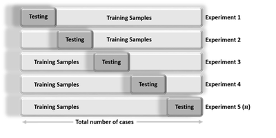
Cross-validation is an iterative process, where each step involves:

• Randomly partitioning a sample of data into 2 complementary subsets (training + testing),

• Performing the analysis on the training subset,

• Validating the analysis on the testing subset

• Increase the iteration index and repeat the process (termination criterial can involve a fixed number, or a desired (mean?) variability or error-rate.

The validation results at each iteration are averaged, to reduce noise/variability, and reported.

Cross-validation guards against testing hypotheses suggested by the data themselves (aka as "Type III errors", False-Suggestion) in cases when new observations are hard to obtain (due to costs, reliability, time or other constraints).

Cross-validation is different from conventional-validation (e.g. 80%-20% partitioning the data set into training and testing subsets) as the in the conventional validation, the error (e.g. Root Mean Square Error, RMSE) on the training data is not a useful estimator of model performance, as it does not generalize across multiple samples. Errors of the conventional-valuation based on the results on the test data do not assess model performance, in general. A more fair way to properly estimate model prediction performance is to use cross-validation, which combines (averages) prediction errors or measures of fit to correct for the stochastic nature of training and testing data partitions and generate a more accurate and robust estimate of real model performance.

A more complex model overfits-the-data, relative to a simpler model when the former generates accurate fitting results for known data but less accurate results when predicting based on new data (foresight). Knowledge from past experience includes information either relevant or irrelevant (noise) for the future information. In challenging data-driven predict models when uncertainty (entropy) is high, more noise is present in past information that needs to be ignored in future forecasting. However it is generally hard to discriminate patterns from noise in complex systems (i.e., deciding which part to model and which to ignore). Models that reduce the chance of fitting noise are called robust.

Example (Linear Regression)

We can demonstrate model assessment using linear regression. Suppose we observe response values {y₁,...,y_n }, and the corresponding k predictors represented as a kD vector of covariates {x₁,...,x_n }, where subjects/cases are indexed by 1 ≤ i ≤ n, and the data-elements (variables) are indexed by 1 ≤ j ≤ k.

((x_1,1&⋯&x_(1,k)@⋮&⋱&⋮@x_(n,1)&⋯&x_(n,k) )) FIX FORMULAS!!!

Using least squares to estimate the linear function parameters (effect-sizes), {β₁,...,β_k}, allows us to compute a hyperplane y = a + xβ that best fits the observed data {x_I,y_I}_{(1 ≤ i ≤ n)}.

FORMULAs!!

(((y_1@⋮)@y_n ))=(((α_1@⋮)@α_n ))+((x_1,1&⋯&x_(1,k)@⋮&⋱&⋮@x_(n,1)&⋯&x_(n,k) ))(((β_1@⋮)@β_k ))

|(y_1=〖α_1+x〗_1,1 β_1+x_1,2 β_2+⋯+x_(1,k) β_k@y_2=〖α_2+x〗_2,1 β_1+x_2,2 β_2+⋯+x_(2,k) β_k@…@y_n=〖α_n+x〗_(n,1) β_1+x_(n,2) β_2+⋯+x_(n,k) β_k )┤

The model fit may be evaluated using the mean squared error (MSE). The MSE for a given value of the parameters α and β on the observed training data {x_I,y_I}_{(1 ≤ i ≤ n)}:

FORMULA!!

MSE= 1/n ∑_(i=1)^n(y_i-⏟(〖〖(α〗_1+x〗_(i,1) β_1+x_(i,2) β_2+⋯+x_(i,k) β_k))┬((predicted value, (y_i ) ̂, at {x_(i,1),…,x_(i,k)}) ) )^2 , vs.

RMSE= √(1/n ∑_(i=1)^n(y_i-⏟(〖〖(α〗_1+x〗_(i,1) β_1+x_(i,2) β_2+⋯+x_(i,k) β_k))┬((predicted value, (y_i ) ̂, at {x_(i,1),…,x_(i,k)}) ) )^2 ).

The expected value of the MSE (over the distribution of training sets) for the training set is FORUMULA!! (n - k - 1)/(n + k + 1) × E, where E is the expected value of the MSE for the testing/validation data. Therefore, fitting a model and computing the MSE on the training set, we will get an over optimistic evaluation assessment (smaller RMSE) of how well the model may fit another dataset. This bias represents in-sample estimate of the fit, whereas we are interested in the cross-validation estimate as an out-of-sample estimate.

In the linear regression model, cross validation is not useful as we can compute the exact correction factor (n - k - 1)/(n + k + 1) and correctly estimate the out-of-sample fit using the (MSE underestimate) in-sample MSE estimate. However, even in this situation, cross-validation remains useful as it can be used to select an optimal regularized cost function.

In most other modeling procedures (e.g. logistic regression), in general, there are no simple closed-form expressions (formulas) to adjust the cross-validation error estimate from the in-sample fit estimate. Cross-validation is generally applicable way to predict the performance of a model on a validation set using stochastic computation instead of obtaining experimental, theoretical, mathematical, or analytic error estimates.

Cross-validation methods

There are 2 classes of cross-validation approaches – exhaustive and non-exhaustive.

Exhaustive cross-validation

Exhaustive cross-validation methods are based on determining all possible ways to divide the original sample into training and testing data. For example, the Leave-m-out cross-validation involves using m observations for testing and the remaining (n-m) observations as training (when m=1, leave-1-out method). This process is repeated on all partitions of the original sample. This method requires model fitting and validating Cⁿ_m times (n is the total number of observations in the original sample and m is the number left out for validation). This requires a very large number of steps¹.

Non-exhaustive cross-validation

Non-exhaustive cross validation methods avoid computing estimates/errors using all possible partitionings of the original sample, but rather approximates these. For example, in the k-fold cross-validation, the original sample is randomly partitioned into k equal sized subsamples. Of the k subsamples, a single subsample is kept as final testing data for validation of the model. The other k - 1 subsamples are used as training data. The cross-validation process is then repeated k times (k folds). Each of the k subsamples is used once as the validation data. There are corresponding k results that are averaged (or otherwise aggregated) to generate a final model-quality estimation. In k-fold validation, all observations are used for both training and validation, and each observation is used for validation exactly once. In general, k is a parameter that needs to be selected by investigator (common values may be 5, 10).

A general case of the k-fold validation is k=n (the total number of observations), when it coincides with the leave-one-out cross-validation.

¹http://www.ohrt.com/odds/binomial.php

A variation of the k-fold validation is stratified k-fold cross-validation, where each fold has the same (approximately) mean response value. For instance, if the model represents a binary classification of cases (e.g., NC vs. PD), this implies that each fold contains roughly the same proportion of the 2 class labels.

Repeated random sub-sampling validation splits randomly the entire dataset into training (where the model is fit) and testing data where the predictive accuracy is assessed). Again, the results are averaged over all iterative splits. This method has an advantage over k-fold cross validation as that the proportion of the training/testing split is not dependent on the number of iterations (folds). However, its drawback is that some observations may never be selected whereas others may be selected multiple-times in the testing/validation subsample, as validation subsets may overlap, and the results will vary each time we repeat the validation protocol (unless we set a seed point in the algorithm).

Asymptotically, as the number of random splits increases, the repeated random sub-sampling validation approaches the leave-k-out cross-validation.

Case-Studies

Example 1: Parkinson’s Diseases Study involving neuroimaging, genetics, clinical, and phenotypic data for over 600 volunteers produced multivariate data for 3 cohorts (HC=Healthy Controls, PD=Parkinson’s, SWEDD= subjects without evidence for dopaminergic deficit).

# update packages

# update.packages()

#load the data: 06_PPMI_ClassificationValidationData_Short.csv

ppmi_data <-read.csv("https://umich.instructure.com/files/330400/download?download_frd=1",header=TRUE)

#binarize the Dx classes

ppmi_data$\$$ResearchGroup <- ifelse(ppmi_data$\$$ResearchGroup == "Control", "Control", "Patient")
attach(ppmi_data)

head(ppmi_data)

# Model-free analysis, classification

# install.packages("crossval")
#library("crossval")
require(crossval)
require(ada)
#set up adaboosting prediction function

#Define a new classification result-reporting function

my.ada <- function (train.x, train.y, test.x, test.y, negative, formula){
    ada.fit <- ada(train.x, train.y)
    predict.y <- predict(ada.fit, test.x)
    #count TP, FP, TN, FN, Accuracy, etc.
    out <- confusionMatrix(test.y, predict.y, negative = negative)
    #negative	 is the label of a negative "null" sample (default: "control").
    return (out)
}

#balance cases

#SMOTE: Synthetic Minority Oversampling Technique to handle class misbalance in binary classification.
set.seed(1000)
#install.packages("unbalanced") to deal with unbalanced group data
require(unbalanced)
ppmi_data$\$$PD <- ifelse(ppmi_data$\$$ResearchGroup=="Control",1,0) 
uniqueID <- unique(ppmi_data$\$$FID_IID) 
 ppmi_data <- ppmi_data[ppmi_data$\$$VisitID==1,]
ppmi_data$\$$PD <- factor(ppmi_data$\$$PD)

colnames(ppmi_data)

#ppmi_data.1<-ppmi_data[,c(3:281,284,287,336:340,341)]
n <- ncol(ppmi_data)
output.1 <- ppmi_data$\$$PD
 
# remove Default Real Clinical subject classifications! 
 ppmi_data$\$$PD <- ifelse(ppmi_data$\$$ResearchGroup=="Control",1,0) 
 input <- ppmi_data[ ,-which(names(ppmi_data) %in% c("ResearchGroup","PD", "X", "FID_IID"))]
 # output <- as.matrix(ppmi_data[ ,which(names(ppmi_data) %in% {"PD"})])
 output <- as.factor(ppmi_data$\$$PD)
c(dim(input), dim(output))

# balance the dataset

data.1<-ubBalance(X= input, Y=output, type="ubSMOTE", percOver=300, percUnder=150, verbose=TRUE)
balancedData<-cbind(data.1$\$$X, data.1$\$$Y)
nrow(data.1$\$$X); ncol(data.1$\$$X)
nrow(balancedData); ncol(balancedData)
nrow(input); ncol(input)

colnames(balancedData) <- c(colnames(input), "PD")

###Check balance

##T test
alpha.0.05 <- 0.05
test.results.bin <- NULL		# binarized/dichotomized p-values
test.results.raw <- NULL		# raw p-values

# get a better error-handling t.test function that gracefully handles NA’s and trivial variances

my.t.test.p.value <- function(input1, input2) {
    obj <- try(t.test(input1, input2), silent=TRUE) 
    if (is(obj, "try-error")) return(NA) else return(obj$\$$p.value)
 } 
 for (i in 1:ncol(balancedData)) 
 {	
     test.results.raw[i]  <- my.t.test.p.value(input[,i], balancedData [,i])
     test.results.bin[i] <- ifelse(test.results.raw[i]  > alpha.0.05, 1, 0)   
     # binarize the p-value (0=significant, 1=otherwise) 
     print(c("i=", i, "var=", colnames(balancedData[i]), "t-test_raw_p_value=", test.results.raw[i]))
 }
 
     #we can also employ (e.g., FDR, Bonferonni) <u>'''correction for multiple testing'''</u>!
     #test.results.corr <- '''stats::p.adjust'''(test.results.raw, method = "fdr", n = length(test.results.raw)) 
     #where methods are "holm", "hochberg", "hommel", "bonferroni", "BH", "BY", "fdr", "none")
     #plot(test.results.raw, test.results.corr)
     #sum(test.results.raw < alpha.0.05, na.rm=T)/length(test.results.raw)  #check proportion of inconsistencies
     #sum(test.results.corr < alpha.0.05, na.rm =T)/length(test.results.corr)
 
#as the sample-size is changed:
 length(input[,5]); length(balancedData [,5])
 #to plot raw vs. rebalanced pairs (e.g., var="L_insular_cortex_Volume"), we need to equalize the lengths
 plot (input[,5] +0*balancedData [,5], balancedData [,5])   # [,5] == "L_insular_cortex_Volume"

 print(c("T-test results: ", test.results))
 #zeros (0) are significant independent between-group T-test differences, ones (1) are insignificant
 
 for (i in 1:(ncol(balancedData)-1)) 
 {
     test.results.raw [i]  <- wilcox.test(input[,i], balancedData [,i])$\$$p.value
    test.results.bin [i] <- ifelse(test.results.raw [i] > alpha.0.05, 1, 0)
    print(c("i=", i, "Wilcoxon-test=", test.results.raw [i]))
}
print(c("Wilcoxon test results: ", test.results.bin))
#test.results.corr <- stats::p.adjust(test.results.raw, method = "fdr", n = length(test.results.raw)) 
#where methods are "holm", "hochberg", "hommel", "bonferroni", "BH", "BY", "fdr", "none")
#plot(test.results.raw, test.results.corr)

#cross validation

#using raw data:
X <- as.data.frame(input); Y <- output
neg <- "1"   # "Control" == "1"

#using Rebalanced data:

X <- as.data.frame(data.1$\$$X); Y <- data.1$\$$Y
#balancedData<-cbind(data.1$\$$X, data.1$\$$Y); dim(balancedData)

#Side note: There is a function name collision for “crossval”, the same method is present in

#the “mlr” (machine Learning in R) package and in the “crossval” package.  
#To specify a function call from a specific package do:  packagename::functionname()

set.seed(115) 
#cv.out <- crossval::crossval(my.ada, X, Y, K = 5, B = 1, negative = neg)
cv.out <- crossval::crossval(my.ada, X, Y, K = 5, B = 1, negative = neg)
    #the label of a negative "null" sample (default: "control")
out <- diagnosticErrors(cv.out$\$$stat) 
 
 print(cv.out$\$$stat)
print(out)

FP	TP	TN	FN
1.0	59.8	23.4	0.2

acc	sens	spec	ppv	npv	lor
0.9857820	0.9966667	0.9590164	0.9835526	0.9915254	8.8531796

#Define a new LDA = Linear discriminant analysis predicting function

require("MASS") # for lda function

predfun.lda = function(train.x, train.y, test.x, test.y, negative)
{   lda.fit = lda(train.x, grouping=train.y)
    ynew = predict(lda.fit, test.x)$\$$class
     #count TP, FP etc.
     out = confusionMatrix(test.y, ynew, negative=negative)
     return( out )
 }

'''(1) a simple example using the sleep dataset''' (containing the effect of two soporific drugs to increase hours of sleep (treatment-compared design) on 10 patients)

 data(sleep)
 X = as.matrix(sleep[,1, drop=FALSE]) # increase in hours of sleep,
     # drop is logical, if TRUE the result is coerced to the lowest possible dimension.
     #The default is to drop if only one column is left, but not to drop if only one row is left.
 Y = sleep[,2] # drug given 
 plot(X ~ Y)
 levels(Y) # "1" "2"
 dim(X) # 20  1

 set.seed(123456)
 cv.out <- '''crossval::crossval'''(predfun.lda, X, Y, K=5, B=20, negative="1")
 cv.out$\$$stat
diagnosticErrors(cv.out$\$$stat)

'''(2) A model-based example (linear regression) using the attitude dataset:''' 

#?attitude, colnames(attitude)

#"rating"     "complaints" "privileges" "learning"   "raises"     "critical"  "advance"

#aggregated survey of clerical employees of an organization, representing 35 employees of 30
 
#(randomly selected) departments. Data=percent proportion of favorable responses to 7 questions in each department.


#Note: when using a data frame, a time-saver is to use “.” to indicate “include all covariates" in the DF. 
 
#E.g., fit <- lm(Y ~ ., data = D)


 data("attitude")
 y = attitude[,1] 		# rating variable
 x = attitude[,-1] 	# date frame with the remaining variables
 is.factor(y)
 summary( lm(y ~ . , data=x) ) 	# R-squared:  0.7326
 #set up lm prediction function

 '''predfun.lm = function(train.x, train.y, test.x, test.y)'''
 {   lm.fit = lm(train.y ~ . , data=train.x)
     ynew = predict(lm.fit, test.x )
     #compute squared error risk (MSE)
     out = mean( (ynew - test.y)^2)
     <span style="background-color: #32cd32">#note that, in general, when fitting linear model to continuous outcome variable (Y),</span>
     <span style="background-color: #32cd32">#we can’t use the '''out<-confusionMatrix(test.y, ynew, negative=negative)''', as it requires a binary outcome</span>
     <span style="background-color: #32cd32">#this is why we use the MSE as an estimate of the discrepancy between observed & predicted values</span> 
     return(out)
 }


#require("MASS")

 '''predfun.lda = function(train.x, train.y, test.x, test.y, negative)'''
 {   lda.fit = lda(train.x, grouping=train.y)
 ynew = predict(lda.fit, test.x)$\$$class
#count TP, FP etc.
out = confusionMatrix(test.y, ynew, negative=negative)
return( out )
}

#prediction MSE using all variables

set.seed(123456)
cv.out.lm = crossval::crossval(predfun.lm, x, y, K=5, B=20, negative="1")
c(cv.out.lm$\$$stat, cv.out.lm$\$$stat.se) 			# 72.581198  3.736784
#reducing to using only two variables
cv.out.lm = crossval::crossval(predfun.lm, x[,c(1,3)], y, K=5, B=20, negative="1")
c(cv.out.lm$\$$stat, cv.out.lm$\$$stat.se)			# 52.563957  2.015109

(3) a real example using the ppmi_data

#ppmi_data <-read.csv("https://umich.instructure.com/files/330400/download?download_frd=1",header=TRUE)
#ppmi_data$\$$ResearchGroup <- ifelse(ppmi_data$\$$ResearchGroup == "Control", "Control", "Patient")
#attach(ppmi_data); head(ppmi_data)
#install.packages("crossval")
#library("crossval")
#ppmi_data$\$$PD <- ifelse(ppmi_data$\$$ResearchGroup=="Control",1,0)
#input <- ppmi_data[ ,-which(names(ppmi_data) %in% c("ResearchGroup","PD", "X", "FID_IID"))]
#output <- as.factor(ppmi_data$\$$PD)

#remove the irrelevant variables (e.g., visit ID)

 output <- as.factor(ppmi_data$\$$PD)
input <- ppmi_data[, -which(names(ppmi_data) %in% c("ResearchGroup","PD", "X", "FID_IID", "VisitID"))]
X = as.matrix(input)	# Predictor variables
Y = as.matrix(output) 	#  Actual PD clinical assessment 
dim(X); dim(Y)

layout(matrix(c(1,2,3,4),2,2)) 		# optional 4 graphs/page
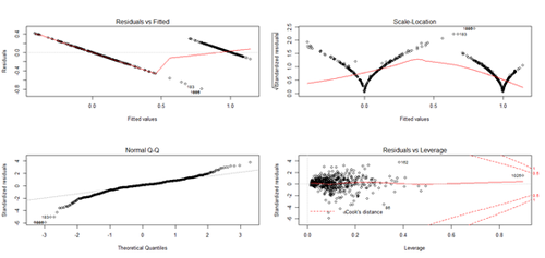
fit <- lm(Y~X); plot(fit)		# plot the fit 
levels(as.factor(Y)) 			# "0" "1"
c(dim(X), dim(Y))			# 1043  103

set.seed(12345)
#cv.out.lm = crossval::crossval(predfun.lm, as.data.frame(X), as.numeric(Y), K=5, B=20)

cv.out.lda = crossval::crossval(predfun.lda, X, Y, K=5, B=20, negative="1")
#K=Number of folds; B=Number of repetitions.

#Results

cv.out.lda$\$$stat; cv.out.lda; diagnosticErrors(cv.out.lda$\$$stat)
cv.out.lm$\$$stat; cv.out.lm; diagnosticErrors(cv.out.lm$\$$stat)

The cross-validation (CV) output object includes the following components:

• stat.cv: Vector od statistics returned by predfun for each cross validation run

• stat: Mean the statistic returned by predfun averaged over all cross validation runs

• stat.se: Variability: the corresponding standard error.

FP	TP	TN	FN
0.06	96.94	33.14	2.06

acc	sens	spec	ppv	npv	lor
0.9839637	0.9791919	0.9981928	0.9993814	0.9414773	10.1655380

Alternative predictor functions

Logistic Regression

(See the earlier batch of class notes, https://umich.instructure.com/files/421847/download?download_frd=1)

#ppmi_data <-
read.csv("https://umich.instructure.com/files/330400/download?download_frd=1",header=TRUE)
# ppmi_data$\$$ResearchGroup <- ifelse(ppmi_data$\$$ResearchGroup == "Control", "Control", "Patient")
#install.packages("crossval"); library("crossval")
#ppmi_data$\$$PD <- ifelse(ppmi_data$\$$ResearchGroup=="Control",1,0)

#remove the irrelevant variables (e.g., visit ID)

output <- as.factor(ppmi_data$\$$PD)
 input <- ppmi_data[, -which(names(ppmi_data) %in% c("ResearchGroup","PD", "X", "FID_IID", "VisitID"))]
 X = as.matrix(input)	# Predictor variables
 Y = as.matrix(output)


<span style="background-color: #32cd32">'''Note that the predicted values are in LOG terms, so we need to exponentiate them to interpret them correctly'''</span>

lm.logit <- glm(as.numeric(Y) ~ ., data = as.data.frame(X), family = "binomial")

ynew <- predict(lm.logit, as.data.frame(X)); plot(ynew)

ynew2 <- ifelse(exp(ynew)<0.5, 0, 1); plot(ynew2)


'''predfun.logit = function(train.x, train.y, test.x, test.y, neg)'''

{ lm.logit <- glm(train.y ~ ., data = train.x, family = "binomial")

<span style="background-color: #32cd32">ynew</span> = predict(lm.logit, test.x )

#compute TP, FP, TN, FN

ynew2 <- ifelse(exp(ynew)<0.5, 0, 1)

out = confusionMatrix(test.y, ynew2, negative=neg)	# Binary outcome, we can use confusionMatrix

return( out )

}

#Reduce the bag of explanatory variables, purely to simplify the interpretation of the analytics in this example!

input.short <- input[, which(names(input) %in% c("R_fusiform_gyrus_Volume",

<blockquote>"R_fusiform_gyrus_ShapeIndex", "R_fusiform_gyrus_Curvedness",
 
"Sex",  "Weight", "Age" , "chr12_rs34637584_GT", "chr17_rs11868035_GT",                                                              
"UPDRS_Part_I_Summary_Score_Baseline", "UPDRS_Part_I_Summary_Score_Month_03",                                             
"UPDRS_Part_II_Patient_Questionnaire_Summary_Score_Baseline",                        

"UPDRS_Part_III_Summary_Score_Baseline",                                             

"X_Assessment_Non.Motor_Epworth_Sleepiness_Scale_Summary_Score_Baseline"</blockquote>    

))]

X = as.matrix(input.short)


cv.out.logit = '''crossval::crossval'''(predfun.logit, as.data.frame(X), as.numeric(Y), K=5, B=2, neg="1")

cv.out.logit$\$$stat.cv

diagnosticErrors(cv.out.logit$\$$stat) <span style="background-color: #32cd32">Caution:</span> Note that if you forget to exponentiate the predicted logistic model values (see ynew2 in predict.logit), you will get nonsense results (e.g., all cases are predicted to be in one class, trivial sensitivity or NPP). predfun.qda = function(train.x, train.y, test.x, test.y, negative) { require("MASS") # for lda function qda.fit = qda(train.x, grouping=train.y) ynew = predict(qda.fit,test.x)$\$$class

out.qda = confusionMatrix(test.y, ynew, negative=negative)

return( out.qda )

}

cv.out.qda = crossval::crossval(predfun.qda, as.data.frame(input.short), as.factor(Y), K=5, B=20, neg="1")

diagnosticErrors(cv.out.lda$\$$stat); diagnosticErrors(cv.out.qda$\$$stat);

This error message: “Error in qda.default(x, grouping, ...) : rank deficiency in group 1” indicates that there is a rank deficiency, i.e. some variables are collinear and one or more covariance matrices cannot be inverted to obtain the estimates in group 1 (Controls)!

If you remove the strongly correlated data elements ("R_fusiform_gyrus_Volume","R_fusiform_gyrus_ShapeIndex", and "R_fusiform_gyrus_Curvedness"), the rank-deficiency problem goes away!

input.short2 <- input[, which(names(input) %in%)"R_fusiform_gyrus_Volume",

"Sex", "Weight", "Age" , "chr17_rs11868035_GT",
"UPDRS_Part_I_Summary_Score_Baseline",
"UPDRS_Part_II_Patient_Questionnaire_Summary_Score_Baseline",
"UPDRS_Part_III_Summary_Score_Baseline",
"X_Assessment_Non.Motor_Epworth_Sleepiness_Scale_Summary_Score_Baseline"

))]

X = as.matrix(input.short2)

cv.out.qda = crossval::crossval(predfun.qda, as.data.frame(X), as.numeric(Y), K=5, B=2, neg="1")

Compare the QDA and GLM/Logit predictions:

diagnosticErrors(cv.out.qda$\$$stat); diagnosticErrors(cv.out.logit$\$$stat)

(default)	Deutsch	Español	Français	Italiano	Português	日本語	България	الامارات العربية المتحدة	Suomi	इस भाषा में	Norge
한국어	中文	繁体中文	Русский	Nederlands	Ελληνικά	Hrvatska	Česká republika	Danmark	Polska	România	Sverige

SMHS BigDataBigSci CrossVal

Contents

Big Data Science - (Internal) Statistical Cross-Validaiton

Questions

Overview

Cross-validation

Overfitting

Example (Linear Regression)

Cross-validation methods

Case-Studies

Alternative predictor functions

See also

Navigation menu

Personal tools

Namespaces

Variants

Views

More

Search

Navigation

Tools