SMHS TimeSeries
Contents
[hide]Scientific Methods for Health Sciences - Time Series Analysis
Overview
Time series data is a sequence of data points measured at successive pints in time spaced intervals. Time series analysis is commonly used in varieties of studies like monitoring industrial processes and tracking business metrics in the business world. In this lecture, we will present a general introduction to the time series data and introduced on some of the most commonly used techniques in the rick and rapidly growing field of time series modeling and analysis to extract meaningful statistics and other characteristics of the data. We will also illustrate the application of time series analysis techniques with examples in R.
Motivation
Economic data like daily share price, monthly sales, annual income or physical data like daily temperature, ECG readings are all examples of time series data. Time series is just an ordered sequence of values of a variable measured at equally spaced time intervals. So, what would be the effective ways to measure time series data? How can we extract information from time series data and make inference afterwards?
Theory
Time series: a sequence of data points measured at successive pints in time spaced intervals.
- Components: (1) trend component: long-run increase or decrease over time (overall upward or downward movement), typically refers to data taken over a long period of time; the trend can be upward or downward, linear or non-linear. (2) seasonal component: short-term regular wave-like patterns, usually refers to data observed within one year, which may be measured monthly or quarterly. (3) cyclical component: long-term wave-like patterns; regularly occur but may vary in length; often measured peak to peak or trough to trough. (4) irregular component: unpredictable, random, ‘residual’ fluctuation, which may be due to random variations of nature or accidents or unusual events; ‘noise’ in the time series.
- Probabilistic models: The components still add or multiply together across time.
- Simple Time Series Models:
- Take $T_{t}$ as the trend component, $S_{t}$ as the seasonal component, $C_{t}$ as the cyclical component and $I_{t}$ as the irregular or random component. Then we have an additive model as: $x_{t}=T_{t}+S_{t}+C_{t}+I_{t};$ the multiplicative model says $x_{t}=T_{t}*S_{t}*C_{t}*I_{t};$ sometimes, we take logs on both sides of the multiplicative model to make it additive, $logx_{t}=log\left ( T_{t}*S_{t}*C_{t}*I_{t} \right )$, which can be further noted as $x_{t}{}'=T_{t}{}'+S_{t}{}'+C_{t}{}'+I_{t}{}'$.
- Most time series models are written in terms of an (unobserved) white noise process, which is often assumed to be Gaussian: $x_{t}=w_{t}$, where $w_{t}\sim WN\left ( 0,1 \right )$, that is, $E\left ( W_{t} \right )=0, Var\left(W_{t} \right )=\sigma ^{2}$. Examples of probabilistic models include: (1) Autoregressive $x_{t}=0.6x_{t-1}+w_{t};$ (2) Moving average model $x_{t}= \frac{1}{3}\left(w_{t}+w_{t-1}+w_{t-2}\right).$
- Fitting time series models: a time series model generates a process whose pattern can then be matched in some way to the observed data; since perfect matches are impossible, it is possible that more than one model will be appropriate for a set of data; to decide which model is appropriate: patterns suggest choices, assess within sample adequacy (diagnostics, tests), outside sample adequacy (forecast evaluation), simulation from suggested model and compare with observed data; next, turn to some theoretical aspects like how to characterize a time series, and then investigate some special processes.
- Characterizing time series (the mean and covariance of time series): suppose the data are $x_{1},x_{2},\cdots ,x_{t},$ note for a regularly spaced time series, $x_{1}$ is observed at time $t_{0}$, $x_{2}$ is observed at $t_{0}+\Delta, x_{t}$ is observed at $t_{0}+\left( t-1\right) \Delta$; the expected value of $x_{t}$ is $\mu _{t}=E\left [ x_{t} \right ]$; the covariance function is $\gamma \left(s,t \right )=cov\left(x_{s},x_{t} \right )$. Note that, we don’t distinguish between random variables and their realizations. Properly, $x_{1},x_{2},\cdots ,x_{t}$ is a realization of some process $X_{1},X_{2},\cdots ,X_{t}$ and so $\mu _{t}=E\left [ x_{t} \right ]$ etc.
- Characterizing time series data: weak stationarity: usually we have only one realization of the time series. There are not enough data to estimate all the means \& covariances. That is if the mean is constant, and the covariance depends only on the separation in time, then a time series is $\left(weakly\right)$ stationary. In this case $\mu_{t}=\mu$ and $\gamma\left(s,t\right)=\gamma\left(t-s\right)$. Stationary processes are much easier to handle statistically. Real time series are usually non-stationary, but can often be transformed to give a stationary process.
- Estimation of $\gamma(h)$ (Estimating the autocovariance function): (1) for a stationary process: $\gamma(h)=\gamma(s,s+h)=cov(x_{s},x_{s+h})$ for any s.$\ \gamma (h)$ is called the autocovariance function because it measures the covariance between lags of the process $x_{t}$; (2) we observe T-h pairs separated at lag h namely $\left(x_{1},x_{h+1}\right),\cdots,\left(x_{T-h},x_{T}\right)$; the sample autocovariance function is $\hat{\gamma}(h)=\frac{1}{T}\sum_{t=1}^{T-h}\left(x_{t}-\bar{X} \right )\left(x_{t+h}-\bar{X} \right )$, note that we divide by ${T}$ although there are ${T-h}$ terms in the sum. The autocorrelation function ${ACF}$ is $\rho (h)=\frac{\gamma(h)}{\gamma(0)}$.
- $\rho(h)$ properties: for $x_{t}$ stationary, $\gamma(h)=E(x_{t}-\mu{t})(x_{t+h}-\mu)$, where $\gamma(h)$ is an even function, that is $\gamma(h)=\gamma(-h); \left | \gamma(h) \right |\leq \left | \gamma(0) \right |$, that is $\left|\rho(h)\right|\leq1, h=\pm 1,2,\cdots$. The autocorrelation matrix, $P(h)$ is positive semi-definite which means that the autocorrelations cannot be chosen arbitrarily but must have some relations among themselves.
- To study a set of time series data: given that we only have one realization, we need to match plot of data from proposed model with data (we can see broad/main patterns); match acf, pacf of proposed model with data (we can see if data are stationary uncorrelated, stationary autocorrelated or non-stationary); determine if the proposed model is appropriate; obtain forecasts from proposed model; compare across models that seem appropriate.
- Large sample distribution of the $ACF$ for a $WN$ series: if $x_{t}$ is $WN$ then for n large, the sample $ACF$, $\hat{\rho}_{x}(h), h=1,2,\cdots$,H where H is fixed but arbitrary is normally distributed with zero mean and standard deviation given by $\sigma_{\hat{\rho}_{x}}(h)=\frac{1}{\sqrt{h}}$. A rule of thumb for assessing whether sample autocorrelations resemble those for a $WN$ series is by checking if approximately 95% of the sample autocorrelations are within the interval $0\pm \frac{2}{\sqrt{n}}$.
- White noise, or stationary uncorrelated process: we say that a time series is white noise if it is weakly stationary, with $ACF$, $\rho(h)=\begin{cases} 1 & \text{ if } h=0 \\ 0 & \text{ if } h> 0\ and\ with \ E\left[w_{t} \right ]=0 \end{cases}$, i.e. white noise consists of a sequence of uncorrelated, zero mean random variables with common variance $\sigma^{2}$.
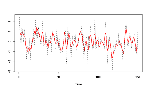
- Example of a simple moving average model in R: $v_{t}=\frac{1}{3} (w_{t-1}+w_{t}+w_{t+1})$.
R CODE:
w <- ts(rnorm(150)) ## generate 150 data from the standard normal distribution
v <- ts(filter(w, sides=2, rep(1/3, 3))) ## moving average model
par(mfrow=c(2,1))
plot(w,main='white noise')
plot(v,main='moving average')
or can use code:
w <- rnorm(150) ## generate 150 data from the standard normal distribution
v <- filter(w, sides=2, rep(1/3, 3)) ## moving average model
par(mfrow=c(2,1))
plot.ts(w,main='white noise')
plot.ts(v,main='moving average')
- sums based on WN processes
ts.plot(w,v,lty=2:1,col=1:2,lwd=1:2)
The ACF and the sample ACF of some stationary processes
- white noise = w(t), acf x(t)=w(t)+\frac{1}{3} \left(w(t-1)+w(t-2)+w(t-3) \right), then plot the barplot of the acf:
RCODE: par(mfrow=c(2,1)) barplot(ARMAacf(0,lag.max=10),main='white noise=w(t)') barplot(ARMAacf(ma=c(1/3,1/3,1/3),lag.max=10),main='acfx(t)=w(t)+1/3w(t-1)+1/3w(t-2)+1/3w(t-3)')
- Theoretical acf of some processes: Autoregressive process, x_{t}=0.9x_{t-1}+w_{t}.
RCODE: par(mfrow=c(2,1))
barplot(ARMAacf(c(0.9),lag.max=30),main='acf x(t)=0.9x(t-1)+w(t)')
barplot(ARMAacf(c(1,-0.9),lag.max=30),main='acf x(t)=x(t-1)-0.9x(t-2)+w(t)')
- Recognizing patterns in probabilistic data
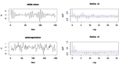
- Example 1: compare White noise & Autoregressive process (x_{t}=w_{t} \& x_{t}=x_{t-1}-0.9x_{t-2}+w_{t})
RCODE:
w1 <- rnorm(200) ## generate 200 data from the standard normal distribution
x <- filter(w1, filter=c(1,-0.9),method='recursive')[-(1:50)]
w2 <- w1[-(1:50)]
xt <- ts(x)
par(mfrow=c(2,2))
plot.ts(w,main='white noise')
acf(w2,lag.max=25)
plot.ts(xt,main='autoregression')
acf(xt,lag.max=25)
- Apparently, there is almost no autocorrelation in white noise, while there is large autocorrelation in second series.
Example 2: AR & MA (x_{t}=x_{t-1}-0.9x_{t-2}+w_{t} \& v_{t}=\frac{1}{3} \left(w_{t-1}+w_{t}+w_{t+1} \right) )
RCODE:
v <- filter(w1, sides=2, rep(1/3, 3))
vt <- ts(v)[2:199]
par(mfrow=c(2,2))
plot.ts(xt,main='white noise')
acf(xt,lag.max=25)
plot.ts(vt,main='autoregression')
acf(vt,lag.max=25)
- ACF, PACF and some examples of data in R
RCODE:
data<- c(28,22,36,26,28,28,26,24,32,30,27,24,33,21,36,32,31,25,24,25,28,36,27,32,34,30,
25,26,26,25,-
44,23,21,30,33,29,27,29,28,22,26,27,16,31,29,36,32,28,40,19,37,23,32,29,-
2,24,25,27,24,16,29,20,28,27,39,23)
par(mfrow=c(1,2))
plot(data)
qqnorm(data)
qqline(data)
data1<-data[c(-31,-55)] par(mfrow=c(1,2)) plot.ts(data1) qqnorm(data1) qqline(data1)
library(astsa)
acf2(data1)
- Examining the data:
Diagnostics of outliers
RCODE: dat<- c(28,22,36,26,28,28,26,24,32,30,27,24,33,21,36,32,31,25,24,25,28,36,27,32,34,30,
25,26,26,25,-44,23,21,30, 33,29, 27,29,28,22,26,27,16,31,29,36,32,28,40,19,
37,23,32,29,-2,24,25,27,24,16,29,20,28,27, 39,23)
plot.ts(dat)
- SOCR Home page: http://www.socr.umich.edu
Translate this page:


