SMHS MethodsHeterogeneity
Scientific Methods for Health Sciences - Methods for Studying Heterogeneity of Treatment Effects, Case-Studies of Comparative Effectiveness Research

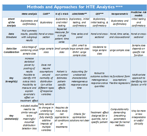
Adopted from: http://dx.doi.org/10.1186/1471-2288-12-185
- *CART: Classification and regression tree (CART) analysis
- ** LGM/GMM: Latent growth modeling/Growth mixture modeling.
- *** QTE: Quantile Treatment Effect.
- **** Standard meta-analysis like fixed and random effect models, and tests of heterogeneity, together with various plots and summaries, can be found in the R-package <bn>rmeta (http://cran.r-project.org/web/packages/rmeta). Non-parametric R approaches are included in the np package, http://cran.r-project.org/web/packages/np/vignettes/np.pdf.
Methods Summaries
Overview
Recursive partitioning is a data mining technique for exploring structure and patterns in complex data. It facilitates the visualization of decision rules for predicting categorical (classification tree) or continuous (regression tree) outcome variables. The R rpart package provides the tools for Classification and Regression Tree (CART) modeling, conditional inference trees, and random forests. Additional resources include an Introduction to Recursive Partitioning Using the RPART Routines . The Appendix includes description of the main CART analysis steps.
install.packages("rpart")
library("rpart")
I. CART (Classification and Regression Tree) is a decision-tree based technique that considers how variation observed in a given response variable (continuous or categorical) can be understood through a systematic deconstruction of the overall study population into subgroups, using explanatory variables of interest. For HTE analysis, CART is best suited for early-stage, exploratory analyses. Its relative simplicity can be powerful in identifying basic relationships between variables of interest, and thus identify potential subgroups for more advanced analyses. The key to CART is its ‘systematic’ approach to the development of the subgroups, which are constructed sequentially through repeated, binary splits of the population of interest, one explanatory variable at a time. In other words, each ‘parent’ group is divided into two ‘child’ groups, with the objective of creating increasingly homogeneous subgroups. The process is repeated and the subgroups are then further split, until no additional variables are available for further subgroup development. The resulting tree structure is oftentimes overgrown, but additional techniques are used to ‘trim’ the tree to a point at which its predictive power is balanced against issues of over-fitting. Because the CART approach does not make assumptions regarding the distribution of the dependent variable, it can be used in situations where other multivariate modeling techniques often used for exploratory predictive risk modeling would not be appropriate – namely in situations where data are not normally distributed.
CART analyses are useful in situations where there is some evidence to suggest that HTE exists, but the subgroups defining the heterogeneous response are not well understood. CART allows for an exploration of response in a myriad of complex subpopulations, and more recently developed ensemble methods (such as Bayesian Additive Regression Trees) allow for more robust analyses through the combination of multiple CART analyses.
Example Fifth Dutch growth study
# Let’s use the Fifth Dutch growth study (2009) fdgs . Is it true that “the world’s tallest nation has stopped growing taller: the height of Dutch children from 1955 to 2009”?
#install.packages("mice")
library("mice")
?fdgs
head(fdgs)
| ID | Reg | Age | Sex | HGT | WGT | HGT.Z | WGT.Z | |
| 1 | 100001 | West | 13.09514 | boy | 175.5 | 75.0 | 1.751 | 2.410 |
| 2 | 100003 | West | 13.81793 | boy | 148.4 | 40.0 | 2.292 | 1.494 |
| 3 | 100004 | West | 13.97125 | boy | 159.9 | 46.5 | 0.743 | 0.783 |
| 4 | 100005 | West | 13.98220 | girl | 159.7 | 46.5 | 0.743 | 0.783 |
| 5 | 100006 | West | 13.52225 | girl | 160.3 | 47.8 | 0.414 | 0.355 |
| 6 | 100018 | East | 10.21492 | boy | 157.8 | 39.7 | 2.025 | 0.823 |
summary(fdgs)
summary(fdgs)
| ID | Reg | Age | Sex | HGT |
| Min.:100001 | North:732 | Min.:0.008214 | boy:4829 | Min.:46.0 |
| 1st Qu.:106353 | East:2528 | 1st Qu.:1.618754 | girl:5201 | 1st Qu.:83.8 |
| Median:203855 | South:2931 | Median:8.084873 | Median:131.5 | |
| Mean:180091 | West:2578 | Mean:8.157936 | Mean:123.9 | |
| 3rd Qu.210591 | City:1261 | 3rd Qu.:13.547570 | 3rd Qu.:162.3 | |
| Max:401955 | Max.:21.993155 | Max.:208.0 | ||
| NA's: 23 |
(1) Classification Tree
Let's use the data frame fdgs to predict Region, from Age, Height, and Weight.
# grow tree
fit.1 <- rpart(reg ~ age + hgt + wgt,   method="class", data= fdgs[,-1])
printcp(fit.1) 	# display the results
plotcp(fit.1) 	# visualize cross-validation results
summary(fit.1) 	# detailed summary of splits
# plot tree
par(oma=c(0,0,2,0))
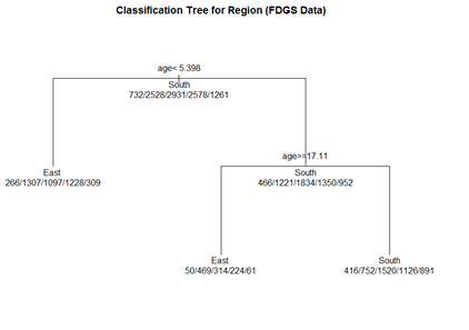
plot(fit.1, uniform=TRUE,  margin=0.3, main="Classification Tree for Region (FDGS Data)")
text(fit.1, use.n=TRUE, all=TRUE, cex=1.0)

# create a better plot of the classification tree
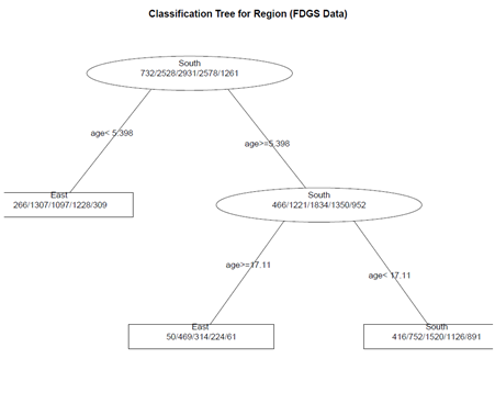
post(fit.1, title = "Classification Tree for Region (FDGS Data)", file = "")

(2) Pruning the tree
pruned.fit.1<- prune(fit.1, cp=   fit.1$\$$cptable[which.min(fit.1$\$$\$$cptable[,"xerror"]),"CP"])

 # plot the pruned tree
 plot(pruned.fit.1, uniform=TRUE,  main="Pruned Classification Tree for Region (FDGS Data)")
 text(pruned.fit.1, use.n=TRUE, all=TRUE, cex=1.0)
 post(pruned.fit.1,  title = "Pruned Classification Tree for Region (FDGS Data)")

Not much change, as the initial tree is not complex!

3) Random Forests

Random forests may improve predictive accuracy by generating a large number of bootstrapped trees (based on random samples of variables). It classifies cases using each tree in this new "forest", and decides the final predicted outcome by combining the results across all of the trees (an average in regression, a majority vote in classification). See the <b>randomForest</b> package.

 library(randomForest)
 fit.2 <- randomForest(reg ~ age + hgt + wgt,   method="class", na.action = na.omit, data= fdgs[,-1])
 print(fit.2) 		# view results
 importance(fit.2) 	# importance of each predictor

Note on missing values/incomplete data: If the data have missing values, we have 3 choices:

1.	Use a different tool (rpart handles missing values well)

2.	Impute the missing values

3.	For a small number of missing cases, we can use na.action = na.omit

==='"`UNIQ--h-2--QINU`"'Latent growth and growth mixture modeling (LGM/GMM)===

LGM and GMM represent structural equation modeling techniques that capture inter-individual differences in longitudinal change corresponding to a particular treatment. For instance, patients’ different timing patterns of the treatment effects may represent the underlying sources of HTE. LGM distinguish if (yes/no) and how (fast/slow, temporary/lasting) patients respond to treatment. The heterogeneous individual growth trajectories are estimated from intra-individual changes over time by examining common population parameters, i.e., slopes, intercepts, and error variances. Suppose each individual has unique initial status (intercept) and response rate (slope) during a specific time interval. Then the variances of the individuals’ baseline measures (intercepts) and changes (slopes) in health outcomes will represent the degree of HTE. The LGM-identified HTE of individual growth curves can be attributed to observed predictors, including both fixed and time varying covariates.

LGM assumes that all individuals are from the same population (too restrictive in some cases). If the HTE is due to observed demographic variables, such as age, gender, and marital status, one may utilize multiple-group LGM. Despite its successful applications for modeling longitudinal change, there may be multiple subpopulations with unobserved heterogeneities. Growth mixture modeling (GMM) extends LGM to allow the identification and prediction of unobserved subpopulations in longitudinal data analysis. Each unobserved subpopulation may constitute its own latent class and behave differently than individuals in other latent classes. Within each latent class, there are also different trajectories across individuals; however, different latent classes don’t share common population parameters. Suppose we are interested in studying retirees’ psychological well-being change trajectory when multiple unknown subpopulations exist. We can add another layer (a latent class variable) on the LGM framework so that the unobserved latent classes can be inferred from the data. The covariates in GMM are designed to affect growth factors distinctly across different latent classes. Therefore, there are two types of HTE: 1) the latent class variable in GMM divides individuals into groups with different growth curves; and 2) coefficient estimates vary across latent classes.

<b>Latent variables</b> are not directly observed – they are inferred (via a model) from other actually observed and directly measured variables. Models that explain observed variables in terms of latent variables are called latent variable models. Then the latent (unobserved) variable is discrete, it’s referred to as <b>latent class variable.</b>

Breast Cancer Example: Recall the LMER package, earlier review discussions, where Linear Mixed Model (LMM) are used for longitudinal data to examine change over time of outcomes according relative to predictive covariates. LMM assumptions include:

(i) continuous longitudinal outcome

(ii) Gaussian random-effects and errors

(iii) linearity of the relationships with the outcome

(iv) homogeneous population

(v) missing at random data

The objectives of LGM/GMM models (see <b>Latent Class Mixed Models, lcmm</b> R package) are to extend the linear mixed model estimation to:

(i)	heterogeneous populations (relax (iv) above). Use <mark><b>hlme</b> for latent class linear mixed models</mark> (i.e. Gaussian continuous outcome)

(ii)	other types of longitudinal outcomes : ordinal, (bounded) quantitative non-Gaussian outcomes (relax (i), (ii), (iii), (iv)). Use <b>lcmm</b> for general latent class mixed models with outcomes of different nature

(iii)	joint analysis of a time-to-event (relax (iv), (v)). Use <b>Jointlcmm</b> for joint latent class models with a longitudinal outcome and a right-censored (left-truncated) time-to-event

Let’s use these data (http://www.ats.ucla.edu/stat/data/hdp.csv), representing cancer phenotypes and predictors (e.g., "IL6", "CRP", "LengthofStay", "Experience") and outcome measures (e.g., remission) collected on patients, nested within doctors (DID) and within hospitals (HID).

We can illustrate the latent class linear mixed models implemented in <b>hlme</b> through a study of the quadratic trajectories of the response (remission) with TumorSize, adjusting for CO2*Pain interaction and assuming correlated random-effects for the functions of SmokingHx and Sex. To estimate the corresponding standard linear mixed model using 1 latent class where CO2 interacts with Pain:

 # install.packages("lcmm")
 library("lcmm")

 hdp <- read.csv("http://www.ats.ucla.edu/stat/data/hdp.csv")
 hdp <- within(hdp, {
 Married <- factor(Married, levels = 0:1, labels = c("no", "yes"))
 DID <- factor(DID)
 HID <- factor(HID)
 })

add a new subject ID column (last column in the data, “ID”), this is necessary for the hmle call
hdp$\$$ID <- seq.int(nrow(hdp))
model.hlme <- hlme(remission ~ IL6 + CRP + LengthofStay + Experience + I(tumorsize^2) + co2*pain + I(tumorsize^2)*pain, random=~ SmokingHx + Sex, subject='ID', data=hdp, ng=1)
summary(model.hlme)
Heterogenous linear mixed model
fitted by maximum likelihood method

hlme(fixed = remission ~ IL6 + CRP + LengthofStay + Experience +
I(tumorsize^2) + co2 * pain + I(tumorsize^2) * pain, random = ~SmokingHx +
Sex, subject = "ID", ng = 1, data = hdp)

Statistical Model:
Dataset: hdp
Number of subjects: 8525
Number of observations: 8525
Number of latent classes: 1
Number of parameters: 21

Iteration process:
Convergence criteria satisfied
Number of iterations:  34
Convergence criteria: parameters= 1.2e-09
: likelihood= 8.3e-06
: second derivatives= 2.7e-05

Goodness-of-fit statistics:
maximum log-likelihood: -5223.9
AIC: 10489.79
BIC: 10637.86
Maximum Likelihood Estimates:
| coef | Se | Wald | p-value | |
| Intercept | 0.28636 | 0.24314 | 1.178 | 0.23890 |
| IL6 | -0.01134 | 0.00183 | -6.184 | 0.00000 |
| CRP | -0.00674 | 0.00167 | -4.043 | 0.00005 |
| LengthofStay | -0.04834 | 0.00463 | -10.436 | 0.00000 |
| Experience | 0.01695 | 0.00119 | 14.263 | 0.00000 |
| I(tumorsize^2) | 0.00000 | 0.00001 | -0.076 | 0.93953 |
| co2 | -0.03549 | 0.16204 | -0.219 | 0.82663 |
| pain | 0.03930 | 0.04278 | 0.919 | 0.35832 |
| co2:pain | -0.01489 | 0.02871 | -0.519 | 0.60395 |
| I(tumorsize^2):pain | 0.00000 | 0.00000 | 0.553 | 0.58045 |
| intercept | SmokingHxformer | SmokingHxnever | Sexmale | |
| intercept | 0.19310943 | |||
| SmokingHxformer | -0.10617988 | 0.209155186 | ||
| SmokingHxnever | -0.12388534 | 0.068342049 | 2.262655e-01 | |
| Sexmale | -0.08130975 | -0.007353491 | -1.873934e-05 | 0.1730187 |
Residual standard error:
coef: 0.1299767
se: 1.187426
Results interpretation:
(1) The first part of the summary provides information about the dataset, the number of subjects, observations, observations deleted (since by default, missing observations are deleted), number of latent classes and number of parameters.
(2) Next, details about the algorithm convergence is provided along with the number of iterations, the convergence criteria, and the information indicating if the model converged correctly: "convergence criteria satisfied".
(3) The maximum log-likelihood, Akaike criterion (AIC) and Bayesian Information criterion (BIC) are reported.
(4) Estimates of parameters, the estimated standard error, the Wald Test statistics (with Normal approximation) and the corresponding p-values are reported below.
(5) For the random-effect distribution, the estimated matrix of covariance of the random-effects is displayed.
(6) The standard error of the residuals is given along with its estimated standard error.
(7) The effect of TumorSize seems not associated with change over Pain of Remission. This may be formally assessed using a multivariate Wald test:
WaldMult(model.hlme, pos=c(6,8))
# pos - a vector containing the indices in model.hlme of the parameters to test
Wald Test p_value
I(tumorsize^2) = pain = 0   0.85562 0.65193
We may consider the model with an adjustment for CRP only on the intercept. Below we estimate the corresponding models for a varying number of latent classes (from 1 to 3) using the default initial values:
# Initial Model: model.hlme <- hlme(remission ~ IL6 + CRP + LengthofStay + Experience + I(tumorsize^2) + co2*pain + I(tumorsize^2)*pain, random=~ SmokingHx + Sex, subject='ID', data=hdp, ng=1)
model.hlme.1 <- hlme(tumorsize ~ IL6 + CRP + LengthofStay, subject='ID', data=hdp, ng=1)
model.hlme.2 <- hlme(tumorsize ~ IL6 + CRP + LengthofStay + SmokingHx, mixture=~ SmokingHx, subject='ID', data=hdp, ng=2)
model.hlme.3 <- hlme(tumorsize ~ IL6 + CRP + LengthofStay + SmokingHx, mixture=~ SmokingHx, subject='ID', data=hdp, ng=3)
The estimation process for a varying number of latent classes can be summarized with summarytable, which gives the log-likelihood, the number of parameters, the Bayesian Information Criterion, and the posterior proportion of each class:
summarytable(model.hlme.1, model.hlme.2, model.hlme.3)
            G    loglik npm      BIC    %class1    %class2  %class3
model.hlme.1 1 -33301.82   5 66648.89 100.000000
model.hlme.2 2 -31592.79  11 63285.15  99.214076  0.7859238
model.hlme.3 3 -31589.55  15 63314.86   6.357771 82.2991202 11.34311
The program took 404.65 seconds)
In this example, the optimal number of latent classes according to the BIC is two (the smallest BIC). The posterior classification is described with:
postprob(model.hlme.2)
Posterior classification:
  class1 class2
N 8458.00  67.00
%   99.21   0.79

Posterior classification table:
    --> mean of posterior probabilities in each class
       prob1  prob2
class1 0.8555 0.1445
class2 0.4362 0.5638

Posterior probabilities above a threshold (%):
        class1 class2
prob>0.7  92.48   2.99
prob>0.8  77.38   0.00
prob>0.9  38.53   0.00
In this example, the first class includes a posteriori 8458 subjects (99%) while class 2 includes 67 (0.79%) subjects. Subjects were classified in class 1 with a mean posterior probability of 0.8555 %.
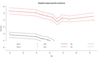
In class 1, 92.48% were classified with a posterior probability above 0.7 while 2.99% of the subjects were classified in class 2 with a posterior probability above 0.7. Goodness-of-fit of the model can be assessed by displaying the residuals as in figure and the mean predictions of the model as in figure, according to the time variable given in var.time:
plot(model.hlme.2)
# Figure (left panel)
plot(model.hlme.2, which="fit", var.time="Age", bty="l", ylab=" Remission ", xlab="Age", lwd=2)
# Figure (right panel)
plot(model.hlme.2, which="fit", var.time="Age", bty="l", ylab=" Remission ", xlab="Age", lwd=2, marg=FALSE)


The latent process mixed models implemented in lcmm are illustrated through the study of the linear trajectory of ntumors with Age adjusted for Sex and assuming correlated random-effects for the intercept and Age. Lines estimate the corresponding latent process mixed model with different link functions:
model.hlme.lin <- lcmm(ntumors ~ Age*Sex, random=~ Age ,subject='ID', data=hdp)
model.hlme.beta <- lcmm(ntumors ~ Age*Sex, random=~ Age, subject='ID', data=hdp, link='beta')
model.hlme.spl <- lcmm(ntumors ~ Age*Sex, random=~ Age, subject='ID', data=hdp, link='splines')
model.hlme.spl5q <- lcmm(ntumors ~ Age*Sex, random=~ Age, subject='ID', data=hdp, link='5-quant-splines')
link function: An optional family of link functions. By default,
- "linear" option specifies a linear link function leading to a standard linear mixed model (homogeneous or heterogeneous as estimated in hlme).
- "beta" for estimating a link function from the family of Beta cumulative distribution functions, "thresholds" for using a threshold model to describe the correspondence between each level of an ordinal outcome and the underlying latent process, and
- "Splines" for approximating the link function by I-splines. For this latter case, the number of nodes and the nodes location should be also specified. The number of nodes is first entered followed by,
- then the location is specified with "equi", "quant" or "manual" for respectively equidistant nodes, nodes at quantiles of the marker distribution or interior nodes entered manually in argument
- intnodes. It is followed by - and finally "splines" is indicated. For example, "7-equi-splines" means I-splines with 7 equidistant nodes, "6-quant-splines" means I-splines with 6 nodes located at the quantiles of the marker distribution and "9-manual-splines" means I-splines with 9 nodes, the vector of 7 interior nodes being entered in the argument intnodes.
summary (model.hlme.lin)
General latent class mixed model fitted by maximum likelihood method

lcmm(fixed = ntumors ~ Age * Sex, random = ~Age, subject = "ID",data = hdp)

Statistical Model:
    Dataset: hdp
    Number of subjects: 8525
    Number of observations: 8525
    Number of latent classes: 1
    Number of parameters: 8
    Link function: linear
Iteration process:
    Maximum number of iteration reached without convergence
    Number of iterations:  100
    Convergence criteria: parameters= 5.4e-10
                        : likelihood= 5.5e-10
                        : second derivatives= 1

Goodness-of-fit statistics:
    maximum log-likelihood: -19915.24
    AIC: 39846.49
    BIC: 39902.89

    Discrete posterior log-likelihood: 0
    Discrete AIC: 16

    Mean discrete AIC per subject: 9e-04
    Mean UACV per subject: 0
    Mean discrete LL per subject: 0

Maximum Likelihood Estimates:

Fixed effects in the longitudinal model:
                             coef Se Wald p-value
intercept (not estimated)  0.00000
Age                        0.09491
Sexmale                   -0.66303
Age:Sexmale                0.01132
Variance-covariance matrix of the random-effects:
          intercept         Age
intercept 20.5013715
Age       -0.2889814 0.007696382
Residual standard error (not estimated) = 1
Parameters of the link function:
                        coef Se Wald p-value
Linear 1 (intercept) -0.36768
Linear 2 (std err)    0.71432
Objects mlin, mbeta, mspl and mspl3eq are latent process mixed models that assume the exact same trajectory for the underlying latent process but respectively a linear, BetaCDF, I-splines with 5 equidistant knots (default with link=’splines’) and I-splines with 5 knots at percentiles. mlin reduces to a standard linear mixed model (link=’linear’ by default). The only difference with a hlme object is the parameterization for the intercept and the residual standard error that are considered as rescaling parameters.
col <- rainbow(4)
plot(model.hlme.lin, which="linkfunction", bty='l', ylab="Number-of-Tumors", col=col[1], lwd=2, xlab="underlying latent process")
plot(model.hlme.beta, which="linkfunction", add=T, col=col[2], lwd=2)
plot(model.hlme.spl, which="linkfunction", add=T, col=col[3], lwd=2)
plot(model.hlme.spl5q, which="linkfunction", add=T, col=col[4], lwd=2)
legend(x="topleft",legend=c("linear", "beta","splines (5equidistant)", "splines (5 at quantiles)"), lty=1,col=col,bty="n",lwd=2)
# to obtain confidence bands use function predictlink
link.lin <- predictlink(model.hlme.lin, ndraws=2000)
Error in predictlink.lcmm(model.hlme.spl, ndraws = 2000):
No confidence intervals can be produced since the program did not converge properly
model.hlme.lin$\$$conv # double-check the convergence of the algorithm[1] 2
# status of convergence:
# =1 if the convergence criteria were satisfied,
# =2 if the maximum number of iterations was reached,
# =4 or 5 if a problem occured during optimisation
model.hlme.lin <- lcmm(ntumors ~ Age*Sex, random=~ Age ,subject='ID', epsY = 0.5, convB = 1e-01, convL = 1e-01, convG = 1e-01, maxiter=200, data=hdp); model.hlme.lin$conv
# Now that we have convergence, we can obtain CI’s!!!
link.lin <- predictlink(model.hlme.lin, ndraws=2000)
# plot(model.hlme.lin, which="linkfunction", bty='l', ylab="Number-of-Tumors", col=col[1], lwd=2, xlab="underlying latent process")
plot(link.lin, add=TRUE, col=col[1], lty=2, lwd=2)
legend(x="left", legend=c("95% confidence bands", "for linear fit"), lty=c(2,NA), col=c(col[1],NA), bty="n", lwd=2)