SMHS LinearModeling LMM Assumptions
Linear mixed effects analyses - Mixed Effect Model Assumptions
First review the Linear mixed effects analyses section.
The same conditions we have in the fixed effect multivariate linear model apply to mixed and random effect models – co-linearity, influential data points, homoscedasticity, and lack of normality. These assumptions can be checked by creating residual plots, histogram plots of the residuals or a Q-Q normal probability plots.
The fixed effect independence condition is relaxed in mixed/random effect models, as this was the main motivation for mixed models – to resolve dependencies in the data. Mixed effect models still require independence, e.g., when ignoring independent and including just a fixed effect for a variable of interest. For instance, working with a model that does not include a random effect “Player”, we have multiple Weight responses per Player. This would violate the LME model independence assumption. Careful selection of fixed effects and random effects is necessary to resolve potential dependencies in the data.
The function dfbeta() can’t be used for assessing influential data points in mixed effects linear models the way it can for fixed effect models. To check for influential points in mixed effect models the package influence.ME15 or a leave-one-out validation can be employed.
For example, we can define a vector of size equal to the number of rows in the data. Iterating over each row (i), we estimate a new mixed model excluding the current row index (data[-i,]). The function fixef() extracts the coefficients of interest, which can be adapted to the specific analysis. Running fixef() on the linear model yields the position of the relevant coefficient. For example, position “1” refers to the intercept (which is always the first coefficient mentioned in the coefficient table) and position “2” reflects the effect of “Height” appears second in the list of coefficients.
df <- as.data.frame(data)
all.res=numeric(nrow(df))
for(i in 1:nrow(df))
{ 		# Generic
# myfullmodel=lmer(response~predictor+ (1+predictor|randomeffect))
# results[i]=fixef(myfullmodel)[parameter position index]
fullmodel=lmer(Weight~Height+ (1+Height|Team), data=data[-i,])
results[i]=fixef(fullmodel)[2]
echo ("Row = ", i)
}
Comments
Fixed effects represent explanatory predictors that are expected to have a systematic and predictable influence on the data (response). Whereas random effects represent covariates expected to have a non-systematic, idiosyncratic, unpredictable, or “random” influence on the response variable. Examples of such random effects in experimental studies include “subject/patient/player/unit” and “Age”, as we generally have no control over idiosyncrasies of individual subjects or their age at time of observation.
Often fixed effects are expected to exhaust the population of interest, or the levels of a factor. In the MLB study the factor “Team” may not exhaust the space as there are other teams/leagues. However, for MLB at a fixed time, the “Team” factor may be fully exhaustive. Same with Height. Random effects represent sub-samples from the population of interest and may not “exhaust” the population as more players or teams could be included in the study. The levels of random factor may only represent a small sub-subset of all levels of the factor.
Hands-on Activity
Use these cancer data (http://www.ats.ucla.edu/stat/data/hdp.csv), representing cancer phenotypes and predictors (e.g., "IL6", "CRP", "LengthofStay", "Experience") and outcome measures (e.g., remission) collected on patients, nested within doctors (DID) and within hospitals (HID). To fit a mixed model (http://www.ats.ucla.edu/stat/r/dae/melogit.htm) and examine remissions as cancer outcomes.
This lung cancer dataset includes a variety of outcomes collected on patients, nested within doctors, who are in turn nested within hospitals. Doctor level variables include experience.
hdp <- read.csv("http://www.ats.ucla.edu/stat/data/hdp.csv")
hdp <- within(hdp, {
Married <- factor(Married, levels = 0:1, labels = c("no", "yes"))
DID <- factor(DID)
HID <- factor(HID)
})
Plot several continuous predictor variables to examine the distributions and catch coding errors (e.g., if values range from 0 to 7, but we see a 999), and explore the relationship among our variables.
# install.packages("ggally")
# library(GGally)
# library("ggplot2")
# ggpairs (hdp[, c("IL6", "CRP", "LengthofStay", "Experience")])
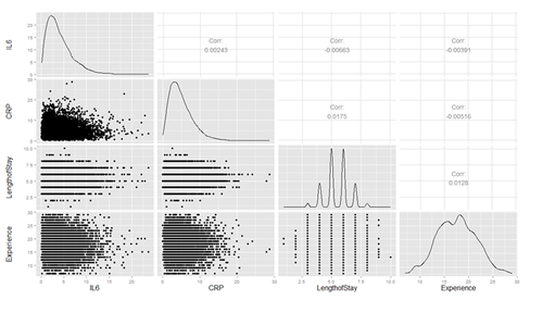
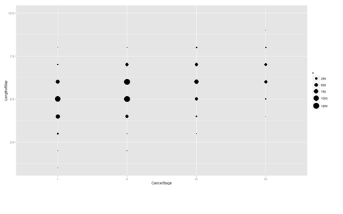
Are there strong linear relations among the continuous variables? Examine CancerStage and LengthofStay closer. The area of bubbles are proportional to the number of observations with the corresponding values.
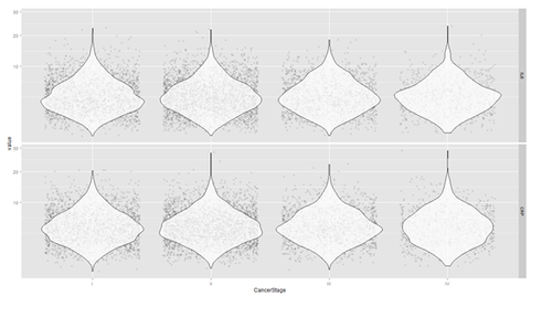
Violin plots may be used for continuous predictors. We can render all raw data separated by CancerStage. To reduce overlaying, we can add some random noise (along the x axis) or alternatively set the alpha opacity level. Note that IL6 and CRP have skewed distributions indicating that we use a square root scale on the y axes. The distributions appear normal and symmetric with long right tails, even after square root transformation.
ggplot(hdp, aes(x = CancerStage, y = LengthofStay)) +
stat_sum(aes(size = ..n.., group = 1)) +
scale_size_area(max_size=10)
# install.packages("reshape")
# library(reshape)
tmp <- melt(hdp[, c("CancerStage", "IL6", "CRP")], id.vars="CancerStage")
ggplot(tmp, aes(x = CancerStage, y = value)) +
geom_jitter(alpha = .1) +
geom_violin(alpha = .75) +
facet_grid(variable ~ .) +
scale_y_sqrt()
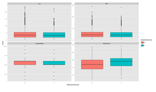
The distribution of continuous variables at each level of the binary outcome to provide a better depiction of the change of the binary variables over levels of continuous variables.
tmp <- melt(hdp[, c("remission", "IL6", "CRP", "LengthofStay", "Experience")], id.vars="remission")
ggplot(tmp, aes(factor(remission), y = value, fill=factor(remission)))+ geom_boxplot() + facet_wrap(~variable, scales="free_y")
Types of Data Analyses16
Mixed effects logistic regression The glmer model can be used to estimate a mixed effects logistic regression model with Il6, CRP, and LengthofStay as patient level continuous predictors, CancerStage as a patient level categorical predictor (I, II, III, or IV), Experience as a doctor level continuous predictor, and a random intercept by DID, doctor ID. Estimating and interpreting generalized linear mixed models (GLMMs, of which mixed effects logistic regression is one) can be quite challenging.
# estimate the model and store results in m
# library("lme4")
m1 <- glmer(remission ~ IL6 + CRP + CancerStage + LengthofStay + Experience +
(1 | DID), data = hdp, family = binomial, control = glmerControl(optimizer = "bobyqa"), nAGQ = 10)
# print the mod results without correlations among fixed effects
print(m1, corr = FALSE)
Generalized linear mixed model fit by maximum likelihood
 (Adaptive Gauss-Hermite Quadrature, nAGQ = 10) [glmerMod]
Family: binomial  ( logit )
This part conforms the estimates (based on an adaptive Gaussian Hermite approximation of the likelihood) using 10 integrations. More integration points improves the approximation (convergnce to the ML estimates), however, increase the computational requirements
To avoid a warning of nonconvergence, we specify a different optimizer with the argument control=glmerControl(optimizer="bobyqa"). Although the model will produce nearly identical results without the new argument, we prefer to use models without such warnings.
Formula: remission ~ IL6 + CRP + CancerStage + LengthofStay + Experience + (1 | DID)
Data: hdp
| AIC | BIC | LogLik | Deviance | df. resid. |
| 7397.276 | 7460.733 | -3689.638 | 7379.276 | 8516 |
Random effects:
| Groups Name | Std. Deviation. |
| DID (Intercept) | 2.015 |
This section gives the basic information to compare models, and lists the random effect estimates. This represents the estimated variability in the intercept on the logit scale. When there are other random effects, e.g., random slopes, they are included here.
The total number of observations, and the number of level 2 observations, the total number of patients (8,525) and doctors (407) are reported.
| (Intercept) | IL6 | CRP | CancerStageII |
| CancerStageIII | CancerStageIV | LengthofStay | Experience |
The part includes a table of the fixed effects estimates. The estimates represent the regression coefficients, which are raw/unstandardized on the logit scale.
The estimates are followed by their standard errors (SEs). As is common in GLMs, the SEs are obtained by inverting the observed information matrix (negative second derivative matrix). However, for GLMMs, this is again an approximation. The approximations of the coefficient estimates likely stabilize faster than do those for the SEs. Thus if you are using fewer integration points, the estimates may be reasonable, but the approximation of the SEs may be less accurate. The Wald tests, Estimate/SE, rely on asymptotic theory, here referring to as the highest level unit size converges to infinity, these tests will be normally distributed, and from that, p values (the probability of obtaining the observed estimate or more extreme, given the true estimate is 0).
To obtain confidence intervals (CIs) using the SE estimates
se <- sqrt(diag(vcov(m1)))
# table of estimates with 95% CI, fixef = Extract fixed-effects estimates
(tab <- cbind(Est = fixef(m1), LL = fixef(m1) - 1.96 * se, UL = fixef(m1) + 1.96 * se))
| Est | LL | UL | |
| (Intercept) | -2.05270650 | -3.09434022 | -1.011072788 |
| IL6 | -0.05677184 | -0.07934785 | -0.034195828 |
| CRP | -0.02148295 | -0.04151100 | -0.001454894 |
| CancerStageII | -0.41393353 | -0.56243063 | -0.265436433 |
| CancerStageIII | -1.00346481 | -1.19609924 | -0.810830385 |
| CancerStageIV | -2.33703403 | -2.64682910 | -2.027238952 |
| LengthofStay | -0.12118216 | -0.18710346 | -0.055260857 |
| Experience | 0.12008900 | 0.06628364 | 0.173894365 |
Instead of coefficients on the logit scale, we can report the add odds ratios by exponentiating the estimates and CIs.
exp(tab)
| Est | LL | UL | |
| (Intercept) | 0.12838695 | 0.04530489 | 0.3638285 |
| IL6 | 0.94480962 | 0.92371856 | 0.9663822 |
| CRP | 0.97874617 | 0.95933878 | 0.9985462 |
| CancerStageII | 0.66104489 | 0.56982235 | 0.7668712 |
| CancerStageIII | 0.36660701 | 0.30237139 | 0.4444888 |
| CancerStageIV | 0.09661377 | 0.07087560 | 0.1316986 |
| LengthofStay | 0.88587258 | 0.82935793 | 0.9462383 |
| Experience | 1.12759721 | 1.06852976 | 1.1899299 |
r1 <- ranef(m1)		# Extract the modes of the random effects
r1.order <- r1[order(r1$\$$DID),]
 # install.packages("lattice")
 dotplot(ranef(m1,condVar=TRUE), lattice.options=list(layout=c(1,2)))

 # Inference
 VarCorr(m1); anova(m1); intervals(m1)

Example of Logistic Regression:

(1)	Logistic curve:

y=f(x)=  <sup>1</sup>⁄<sub>1+e<sup>-x1</sup></sub>

where <i>y</i> and <i>x</i> represent probability and quantitative-predictor values, respectively.

 x <- seq(-10,10,1)
 plot(x,1/(1+exp(-x)), type="l")

<center>[[Image:SMHS_LinearModeling_Fig39.png|500px]]</center>

The point of this logistic curve is:

y= <sup>1</sup>⁄<sub>1+e<sup>x-1</sup></sub> ⇔ x=ln(<sup>y</sup>⁄<sub>1-y</sub>)

which is the log-odds (when y is the probability of an event of interest)

(2)	Logistic regression equation model to estimate the probability of specific outcomes:

MISSING FORMULA ------ (Estimate of)P(Y=1 | x<sub>1</sub>, x<sub>2</sub>,...,x<sub>1</sub> = -----------MISSING FORMULA ------

the coefficients a<sub>o</sub>,  (intercept) and a<sub>k,</sub> k = 1,2,...,l, are estimated using GLM according to a maximum likelihood approach. Using this model allows us to estimate the probability of the dependent (outcome) variable Y=1 (CO), i.e., surviving surgery, given the observed values of the predictors X<sub>k,</sub>k = 1,2,...,l.

Probability of surviving a heart transplant based on surgeon’s experience. A group of 20 patients undergo heart transplantation with different surgeons having experience in the range {0(least), 2…, 10(most)}, representing 100’s of operating/surgery hours. How does the surgeon’s experience affect the probability of the patient survival?

The data is shown below and represents each patient and the outcome of the surgery (1=survival) or (0=death).

<center>
{| class="wikitable" style="text-align:center; width:35%" border="1"

|-
|Surgeon's Experience||1||1.5||2||2.5||3||3.5||3.5||4||4.5||5||5.5||6||6.5||7||8||8.5||9||9.5||10||10
|-
|Clinical Outcome||0||0||0||0||0||0||1||0||1||0||1||0||1||0||1||1||1||1||1||1
|}
</center>


 mydata <- read.csv('https://umich.instructure.com/files/405273/download?download_frd=1&verifier=AOny2eq3wF7WqWAV5YsT6e9zakRTEbZpcuNYRdtM')  # 01_HeartSurgerySurvivalData.csv
 # estimates a logistic regression model for the clinical outcome (CO), survival, using the glm
 # (generalized linear model) function.
 # convert Surgeon’s Experience (SE) to a factor to indicate it should be treated as a categorical variable.
 # mydata$\$$rank <- factor(mydata$\$$SE)
mylogit <- glm(CO ~ SE, data = mydata, family = "binomial")
# library(ggplot2)
ggplot(mydata, aes(x=SE, y=CO)) + geom_point() +
 		stat_smooth(method="glm", family="binomial", se=FALSE)
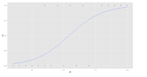
Graph of a logistic regression curve showing probability of surviving the surgery versus surgeon’s experience.
The graph shows the probability of the clinical outcome, survival, (Y-axis) versus the surgeon’s experience (X-axis), with the logistic regression curve fitted to the data.
mylogit <- glm(CO ~ SE, data = mydata, family = "binomial")
summary(mylogit)
The logistic regression analysis gives the following output.
| Estimate Std. | Error | z value | Pr (>z) Wald | |
| (Intercept) | -4.1030 | 1.7629 | -2.327 | 0.0199 * |
| SE | 0.7583 | 0.3139 | 2.416 | 0.0157 * |
The output indicates that surgeon’s experience (SE) is significantly associated with the probability of surviving the surgery (0.0157, Wald test). The output also provides the coefficients for:
Intercept = -4.1030 and SE = 0.7583.
SE=2; CO =1/(1+exp(-(-4.1030+0.7583*SE)))
> CO
[1] 0.07001884
SE=4; CO =1/(1+exp(-(-4.1030+0.7583*SE))); CO
> CO
[1] 0.2554411
The table below shows the probability of surviving surgery for several values of surgeons’ experience.
| Surgeon's Experience | Probability of Patient Survival (Clinical Outcome) |
| 1 | 0.034 |
| 2 | 0.07 |
| 3 | 0.14 |
| 4 | 0.26 |
| 5 | 0.423 |
The output from the logistic regression analysis gives a p-value of p=0.0157, which is based on the Wald z-score. In addition to the Wald method, we can calculate the p-value for logistic regression (mylogit <- glm(CO ~ SE,data = mydata,family = "binomial")) using the Likelihood Ratio Test (LRT), which for these data give 0.0006476922.
| Estimate Std. | Error | z value | Pr (>z) Wald | |
| SE | 0.7583 | 0.3139 | 2.416 | 0.0157 * |
The logit of a number 0≤p≤1 given by the formula: logit(p) = log(p⁄1-p), representing the log-odds (of survival in this case).
confint(mylogit)
So, why exponentiating the coefficients? Because,
Missing Formula--------------
> exp(coef(mylogit)) 	 # exponentiated logit model coefficients
(Intercept)          	SE
0.01652254  		2.13474149   ## == exp(0.7583456)
> coef(mylogit)    	# raw logit model coefficients
(Intercept)          	SE
-4.1030298   		0.7583456
exp(cbind(OR = coef(mylogit), confint(mylogit)))
| OR | 2.5% | 97.5% | |
| (Intercept) | 0.01652254 | 0.0001825743 | 0.277290 |
| SE | 2.13474149 | 1.3083794719 | 4.839986 |
with(mylogit, df.null - df.residual)
Finally, the LRT (likelihood-ratio test) p-value can be obtained using:
with(mylogit, pchisq(null.deviance - deviance, df.null - df.residual, lower.tail = FALSE))
[1] 0.0006476922
The LRT p_value < 0.001 tells us that our model as a whole fits significantly better than an empty model. The deviance residual is -2*log likelihood, and to see the model's log likelihood:
logLik(mylogit)
'log Lik.' -8.046117 (df=2)
Side-note: The LRT compares the data fit of two models. For instance, removing predictor variables from a model will reduce model quality (i.e., a model will have a lower log likelihood). To statistically assess whether the observed difference in model fit is significant, the LRT compares the difference of the log likelihoods of the two models. When this difference is statistically significant, the full model (the one with more variables) is a better fit to the data, compared to the reduced model. LRT is computed from the log likelihoods of the models:
MISSING FORMULA------------
m1 and m2 are the reduced and the full models, respectively, L(m1) and L(m2) denote the likelihoods of the 2 models, and ll(m1) and ll(m2) represent the log likelihood (natural log of the model likelihood.
The distribution of the LRT is chi-squared with degrees of freedom equal to the number of parameters that are reduced (i.e., the number of variables removed from the model). In our case,
MISSING FORMULA----- as we have an intercept and one predictor (SE), and the null model is empty (no parameters).
15 http://cran.r-project.org/web/packages/influence.ME/influence.ME.pdf
16 http://www.ats.ucla.edu/stat/mult_pkg/glmm.htm
Next See
Machine Learning Algorithms section for data modeling, training , testing, forecasting, prediction, and simulation.
- SOCR Home page: http://www.socr.umich.edu
Translate this page: