AP Statistics Curriculum 2007 Laplace
Contents
General Advance-Placement (AP) Statistics Curriculum - Laplace Distribution
Laplace Distribution
Definition: Laplace distribution is a distribution that is symmetrical and more “peaky” than a normal distribution. The dispersion of the data around the mean is higher than that of a normal distribution. Laplace distribution is also sometimes called the double exponential distribution.
Probability density function: For \(X\sim \operatorname{Laplace}(\mu,b)\), the Laplace probability density function is given by
\[\frac{1}{2b}\exp(-\frac{|x-\mu|}{b})\]
where
- e is the natural number (e = 2.71828…)
- b is a scale parameter (determines the profile of the distribution)
- \(\mu\) is the mean
- x is a random variable
Cumulative density function: The Laplace cumulative distribution function is given by
\[ \left\{\begin{matrix} \frac{1}{2}\exp(\frac{x-\mu}{b}) & \mbox{if }x < \mu \\[8pt] 1-\frac{1}{2}\exp(-\frac{x-\mu}{b}) & \mbox{if }x \geq \mu \end{matrix}\right. \]
where
- e is the natural number (e = 2.71828…)
- b is a scale parameter (determines the profile of the distribution)
- \(\mu\) is the mean
- x is a random variable
Moment generating function: The Laplace moment-generating function is
\[M(t)=\frac{\exp(\mu t)}{1-b^2 t^2} \mbox{ for }|t|<\frac{1}{b}\]
Expectation:
\[E(X)=\mu\!\]
Variance: The gamma variance is
\[Var(X)=2b^2\!\]
Related Distributions
- If \(X\sim \operatorname{Laplace}(\mu,b)\!\), then \(kX+b\sim \operatorname{Laplace}(k\mu+b,kb)\!\)
- If \(X \sim \operatorname{Laplace}(0,b)\!\), then \(|X| \sim \operatorname{Exponential}(\tfrac{1}{b})\!\) ([Exponential distribution])
- If \(X \sim \operatorname{Exponential}(\tfrac{1}{\lambda})\!\) and \(Y \sim \operatorname{Exponential}(\tfrac{1}{\lambda})\!\), then \(X-Y \sim \operatorname{Laplace}\left(0,\lambda\right)\!\)
- If \(X \sim \operatorname{Laplace}(\mu,\tfrac{1}{b})\!\), then \(|X-\mu| \sim \operatorname{Exponential}(b)\!\)
- If \(X_i \sim \operatorname{Normal}(0,1)\!\) for \(i={1,2,3,4}\!\) then \(X_1 X_2 - X_3 X_4 \sim \operatorname{Laplace}(0,1)\!\) ([Normal distribution])
- If \(X_i \sim \operatorname{Normal}(0,1)\!\) for \(i={1,2,3,4}\!\), then \(X_1 X_2 + X_3 X_4 \sim \operatorname{Laplace}(0,1)\!\)
- If \(X_i \sim \operatorname{Laplace}(\mu,b)\!\), then \(\frac{2}{b \sum_{i=1}^n |X_i-\mu|} \sim \chi^2(2n) \! \) ([Chi-square distribution])
- If \(X \sim \operatorname{Laplace}(\mu,b)\) and \(Y \sim \operatorname{Laplace}(\mu,b)\), then \( \tfrac{|X-\mu|}{|Y-\mu|} \sim \operatorname{F}(2,2) \) ([F-distribution])
- If \(X \sim \operatorname{U}(0,1)\!\) and \(Y \sim \operatorname{U}(0,1)\!\), then \(\log{\tfrac{X}{Y}} \sim \operatorname{Laplace}(0,1)\!\) ([Uniform distribution])
- If \(X \sim \operatorname{Exponential}(\lambda)\!\) and \(Y \sim \operatorname{Bernoulli}(0.5)\!\) independent of \(X\!\), then \( X(2Y-1) \sim \operatorname{Laplace} (0,\lambda^{-1}) \!\)([Bernoulli distribution])
- If \(X_1 \sim \operatorname{Exponential}(\lambda_1)\!\) and \(X_2 \sim \operatorname{Exponential}(\lambda_2)\!\) independent of \(X_1\!\), then \(\lambda_1 X_1-\lambda_2 X_2 \sim \operatorname{Laplace}\left(0,1\right)\,\)
- If \(V \sim \operatorname{Exponential}(1)\!\) and \( Z \sim \operatorname{Normal}(0,1)\, \) independent of \(V\), then \(X = \mu + b \sqrt{2 V}Z \sim \operatorname{Laplace}(\mu,b)\)
Relation to exponential distribution: A Laplace random variable can be represented as the difference of two independent and identically distributed exponential random variables. One way to show is this by using the characteristic function approach.
Consider to independent and identically distributed random variables \(X_1,X_2\sim \operatorname{Exponential}(\lambda)\!\). The characteristic functions for \(X_1-X_2\) are \(\tfrac{\lambda}{-it+\lambda}\) and \(\tfrac{\lambda}{it+\lambda}\) respectively. The product of these two functions is equivalent to the characteristic function of the sum of the random variables \(X_1+(-X_2)\). The result is \(\tfrac{\lambda^2}{(-it+\lambda)(it+\lambda)} =\tfrac{\lambda^2}{t^2+\lambda^2}\).
This is the same as the characteristic function for \(Y\sim\operatorname{Laplace}(0,\tfrac{1}{\lambda})\), which is \(\tfrac{1}{1+\tfrac{t^2}{\lambda^2}}\)
Applications
The Laplace distribution is used for modeling in signal processing, various biological processes, finance, and economics. Examples of events that may be modeled by Laplace distribution include:
- Credit risk and exotic options in financial engineering
- Insurance claims
- Structural changes in switching-regime model and Kalman filter
Example
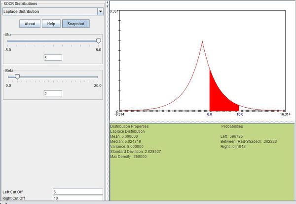
Suppose that the return of a certain stock has a Laplace distribution with \(\mu=5\) and \(b=2\). Compute the probability that the stock will have a return between 6 and 10.
We can compute this as follows:
\[P(6 \le X\le 10)=\sum_{x=6}^{10}\frac{1}{2\times 2}\exp(-\frac{|x-5|}{2})=0.262223\]
The figure below shows this result using SOCR distributions

- SOCR Home page: http://www.socr.ucla.edu
Translate this page: