SOCR EduMaterials Activities BMI Modeling Activity

SOCR Educational Materials - Activities - SOCR Body Mass Index (BMI) Activity and Applications of the Chi-Squared Test

Often times when solving a problem from intro-level textbooks, we are told to assume that a population follows a normal distribution. Other times, a graph of the data will allow us to assume some degree of normality. This allows the use of a number of statistical analyses later on.

Motivation and Goals

The following activity will demonstrate one of the ways to test for normality, using the Chi-Squared test for Goodness-of-Fit. The model to fit will be the normal model. We will run this test on a human characteristic often assumed to fit at least some kind of normal model: BMI.

Summary

This activity uses a simplified version of the BMI data sets found here. Four cases of data were excluded due to extremely high BMIs that hinted at a mistake in the entry process. 10 variables from the original dataset were left out in the dataset presented here, though the same process presented here may be used on them for additional practice.

Data

Data Description

• Number of cases: 248
• Variables
  • Underwater Density – Density determined via a graduated-cylinder type test
  • Body fat—Calculated body density and tissue-type proportions using Siri’s equation (see the full dataset page)
  • Height
  • Weight
  • BMI—Body Mass Index, calculated as \( \frac{weight}{height^2} \).

Data Summary

Statistic	Underwater_Density_(\( \frac{g}{cm^3}\))	Body_Fat	Height(m)	Weight_(kg)	BMI
Mean	1.0562	18.854	1.787	80.547	25.18643319
SD	0.0184	8.0663	0.0659	12.0076	3.146481308

Raw Dataset

Underwater_Density(g/cm3)	Body_Fat	Height(m)	Weight(kg)	BMI
1.0708	12.3	1.72085	69.96662	23.6268
1.0853	6.1	1.83515	78.58488	23.33436
1.0414	25.3	1.68275	69.85322	24.66876
1.0751	10.4	1.83515	83.80119	24.88325
1.034	28.7	1.80975	83.57439	25.51738
1.0502	20.9	1.89865	95.3678	26.45525
1.0549	19.2	1.77165	82.10022	26.15703
1.0704	12.4	1.8415	79.83226	23.54155
1.09	4.1	1.8796	86.63614	24.5227
1.0722	11.7	1.8669	89.92469	25.80102
1.083	7.1	1.8923	84.48158	23.59294
1.0812	7.8	1.9304	97.97595	26.29208
1.0513	20.8	1.7653	81.87342	26.27277
1.0505	21.2	1.80975	93.09983	28.42574
1.0484	22.1	1.7653	85.16197	27.32805
1.0512	20.9	1.6764	73.82216	26.26827
1.0333	29	1.8034	88.79071	27.3013
1.0468	22.9	1.8034	94.9142	29.18415
1.0622	16	1.72085	83.3476	28.14538
1.061	16.5	1.8669	96.04818	27.55796
1.0551	19.1	1.7272	81.19303	27.21658
1.064	15.2	1.77165	90.94527	28.97505
1.0631	15.6	1.73355	63.61633	21.16878
1.0584	17.7	1.778	67.47187	21.34319
1.0668	14	1.72085	68.60585	23.16728
1.0911	3.7	1.8161	72.23458	21.90109
1.0811	7.9	1.7145	59.6474	20.29161
1.0468	22.9	1.7145	67.13167	22.83771
1.091	3.7	1.64465	60.44118	22.34529
1.079	8.8	1.7526	72.91497	23.73838
1.0716	11.9	1.87325	82.55381	23.52587
1.0862	5.7	1.80975	72.68818	22.19354
1.0719	11.8	1.80975	76.20352	23.26686
1.0502	21.3	1.8034	99.10993	30.47425
1.0263	32.3	1.8669	112.1507	32.17806
1.0101	40.1	1.651	86.97634	31.90854
1.0438	24.2	1.778	91.73906	29.01956
1.0346	28.4	1.73355	89.2443	29.69667
1.0258	32.6	1.7018	92.07925	31.79397
1.0279	31.6	1.778	98.42954	31.13594
1.0269	32	1.8161	96.16158	29.15561
1.0814	7.7	1.7272	56.81244	19.044
1.067	13.9	1.86055	74.50255	21.52229
1.0742	10.8	1.7145	60.55458	20.60023
1.0665	5.6	1.80975	67.35847	20.56625
1.0678	13.6	1.7399	61.57516	20.34028
1.0903	4	1.69545	57.83303	20.11898
1.0756	10.2	1.83515	71.78099	21.31407
1.084	6.6	1.7526	63.16274	20.56342
1.0807	8	1.72085	62.25555	21.02287
1.0848	6.3	1.8669	69.28623	19.87947
1.0906	3.9	1.7145	61.80196	21.02458
1.0473	22.6	1.8288	89.81129	26.85335
1.0524	20.4	1.7272	82.32702	27.5967
1.0356	28	1.7653	91.28546	29.29305
1.028	31.5	1.79705	91.85245	28.44267
1.043	24.6	1.67005	81.53323	29.23316
1.0396	26.1	1.86055	97.97595	28.30328
1.0317	29.8	1.7399	81.07964	26.78325
1.0298	30.7	1.78435	87.65673	27.5312
1.0403	25.8	1.7018	80.73944	27.87845
1.0264	32.3	1.778	93.21323	29.48588
1.0313	30	1.7145	83.2342	28.31567
1.0499	21.5	1.79705	68.71924	21.27933
1.0673	13.8	1.8161	70.19342	21.28222
1.0847	6.3	1.75895	70.42022	22.76095
1.0693	12.9	1.8161	71.1006	21.55727
1.0439	24.3	1.8161	75.97672	23.03568
1.0788	8.8	1.74625	66.56468	21.82886
1.0796	8.5	1.87325	72.91497	20.77903
1.068	13.5	1.6256	56.69905	21.45598
1.072	11.8	1.67005	64.86371	23.25642
1.0666	18.5	1.7145	67.24507	22.87628
1.079	8.8	1.7653	73.70876	23.65277
1.0483	22.2	1.7399	80.62604	26.63341
1.0498	21.5	1.78435	73.14177	22.97235
1.056	18.8	1.75895	77.67769	25.10668
1.0283	31.4	1.72085	74.27575	25.08193
1.0382	26.8	1.70815	68.15225	23.3576
1.0568	18.4	1.84785	86.29595	25.27301
1.0377	27	1.778	77.4509	24.49982
1.0378	27	1.75895	76.20352	24.63021
1.0386	26.6	1.7145	75.74993	25.76958
1.0648	14.9	1.70815	71.5542	24.52354
1.0462	23.1	1.67005	72.57478	26.02117
1.08	8.3	1.8415	80.17245	23.64186
1.0666	14.1	1.8542	79.83226	23.22016
1.052	20.5	1.778	80.28585	25.3966
1.0573	18.2	1.7653	81.53323	26.16361
1.0795	8.5	1.7907	74.95614	23.37553
1.0424	24.9	1.82245	87.31653	26.28968
1.0785	9	1.8923	83.57439	23.33959
1.0991	17.4	1.97485	101.8315	26.11042
1.077	9.6	1.86055	85.61556	24.73261
1.073	11.3	1.6891	73.70876	25.83499
1.0582	17.8	1.73355	70.98721	23.62149
1.0484	22.2	1.8288	89.3577	26.71773
1.0506	21.2	1.8669	90.03809	25.83355
1.0524	20.4	1.8288	78.81167	23.56449
1.053	20.1	1.80975	78.35808	23.92471
1.048	22.3	1.87325	89.2443	25.4325
1.0412	25.4	1.75895	80.28585	25.94968
1.0578	18	1.7399	75.06954	24.79792
1.0547	19.3	1.8669	90.83187	26.0613
1.0569	18.3	1.88595	92.19265	25.92006
1.0593	17.3	1.9177	87.99692	23.92799
1.05	21.4	1.75895	76.43031	24.70351
1.0538	19.7	1.7399	77.4509	25.58456
1.0355	28	1.778	83.1208	26.29337
1.0486	22.1	1.778	80.85284	25.57595
1.0503	21.3	1.78435	73.93556	23.22166
1.0384	26.7	1.82245	79.49206	23.93385
1.0607	16.7	1.75895	71.66759	23.16412
1.0529	20.1	1.84785	80.39925	23.54608
1.0671	13.9	1.8288	81.19303	24.27651
1.0404	25.8	1.8796	86.63614	24.5227
1.0575	18.1	1.83515	85.04857	25.25363
1.0358	27.9	1.8923	93.66682	26.15808
1.0414	25.3	1.8161	84.02799	25.47678
1.0652	14.7	1.74625	72.68818	23.83696
1.0623	16	1.69545	68.71924	23.90608
1.0674	13.8	1.6891	73.02837	25.59652
1.0587	17.5	1.7018	75.74993	26.15563
1.0373	27.2	1.74625	80.51265	26.40288
1.059	17.4	1.72085	69.05944	23.32046
1.0515	20.8	1.86055	87.20313	25.19123
1.0648	14.9	1.77165	74.95614	23.88094
1.0575	18.1	1.8161	77.90449	23.62017
1.0472	22.7	1.7907	77.67769	24.22427
1.0452	23.6	1.86055	89.3577	25.81364
1.0398	26.1	1.69545	71.214	24.77396
1.0435	24.4	1.7653	76.31692	24.48972
1.0374	27.1	1.77165	84.36818	26.8796
1.0491	21.8	1.79705	75.63653	23.42131
1.0325	29.4	1.8796	85.16197	24.10543
1.0481	22.4	1.80975	76.31692	23.30149
1.0522	20.4	1.905	96.50178	26.59165
1.0422	24.9	1.8034	80.17245	24.65137
1.0571	18.3	1.7653	78.58488	25.2175
1.0459	23.3	1.72085	75.74993	25.57974
1.0775	9.4	1.83515	72.46138	21.5161
1.0754	10.3	1.9685	85.3434	22.02415
1.0664	14.2	1.79705	70.76041	21.91139
1.055	19.2	1.84785	94.57401	27.69736
1.0322	29.6	1.77165	93.66682	29.84214
1.0873	5.3	1.8415	65.2039	19.22782
1.0416	25.2	1.78435	101.1511	31.76951
1.0776	9.4	1.7526	69.05944	22.48316
1.0542	19.6	1.8923	109.656	30.62333
1.0758	10.1	1.83515	66.22449	19.66416
1.061	16.5	1.70815	71.1006	24.36808
1.051	21	1.8669	90.83187	26.0613
1.0594	17.3	1.91135	77.79109	21.29362
1.0287	31.2	1.7526	93.32663	30.38365
1.0761	10	1.83515	82.78061	24.5802
1.0704	12.5	1.74625	61.91536	20.30419
1.0477	22.5	1.8161	80.39925	24.37656
1.0775	9.4	1.83515	68.60585	20.37127
1.0653	14.6	1.8542	88.9041	25.85882
1.069	13	1.74625	83.57439	27.40693
1.0644	15.1	1.7907	63.50293	19.80378
1.037	27.3	1.8288	99.22333	29.66753
1.0549	19.2	1.87325	98.42954	28.05007
1.0492	21.8	1.7272	75.40973	25.27797
1.0525	20.3	1.83515	101.9449	30.27069
1.018	34.3	1.7653	103.5325	33.22306
1.061	16.5	1.7653	78.35808	25.14472
1.0926	3	1.72085	69.05944	23.32046
1.0983	0.7	1.6637	57.03924	20.60742
1.0521	20.5	1.8034	80.39925	24.7211
1.0603	16.9	1.8161	79.94566	24.23904
1.0414	25.3	1.82245	102.8521	30.9672
1.0763	9.9	1.75895	65.88429	21.29486
1.0689	13.1	1.7018	68.49245	23.6497
1.0316	29.9	1.8161	109.4292	33.17827
1.0477	22.5	1.75895	84.93517	27.45242
1.0603	16.9	1.8923	106.4808	29.7366
1.0387	26.6	1.88595	99.45013	27.9605
1.1089	0	1.7272	53.7507	18.01768
1.0725	11.5	1.70815	66.11109	22.65804
1.0713	12.1	1.77165	72.23458	23.01385
1.0587	17.5	1.88595	77.3375	21.74352
1.0794	8.6	1.8161	75.97672	23.03568
1.0453	23.6	1.88595	105.5736	29.68212
1.0524	20.4	1.8288	95.48119	28.54864
1.052	20.5	1.8415	91.73906	27.05271
1.0434	24.4	1.73355	83.91459	27.92317
1.0728	11.4	1.75895	69.39963	22.43108
1.014	38.1	1.9304	110.7899	29.73073
1.0624	15.9	1.7907	87.77012	27.37165
1.0429	24.7	1.89865	101.9449	28.27976
1.047	22.8	1.84785	73.82216	21.61988
1.0411	25.5	1.73355	81.64663	27.16849
1.0488	22	1.7526	70.87381	23.07386
1.0583	17.7	1.8161	76.20352	23.10444
1.0841	6.6	1.84785	75.86332	22.21767
1.0462	23.6	1.7145	77.4509	26.34823
1.0709	12.2	1.78435	80.85284	25.39424
1.0484	22.1	1.75895	68.03886	21.99126
1.034	28.7	1.8161	90.94527	27.57405
1.0854	6	1.8796	83.461	23.62396
1.0209	34.8	1.77165	101.1511	32.22662
1.061	16.6	1.8542	94.68741	27.54096
1.025	32.9	1.6637	75.29633	27.20344
1.0254	32.8	1.8415	88.45051	26.08296
1.0771	9.6	1.78435	72.80158	22.8655
1.0742	10.8	1.79705	72.46138	22.43811
1.0829	7.1	1.7272	63.72973	21.36273
1.0373	27.2	1.8923	98.08935	27.39314
1.0543	19.5	1.82245	76.31692	22.97786
1.0561	18.7	1.79705	88.33711	27.35413
1.0543	19.5	1.8542	78.35808	22.79138
1.0678	13.6	1.77165	67.69866	21.56871
1.0819	7.5	1.778	70.08002	22.16821
1.0433	24.5	1.82245	90.37828	27.21152
1.0646	15	1.75895	70.08002	22.65099
1.0706	12.4	1.7907	69.51303	21.67807
1.0399	26	1.83515	104.3262	30.97778
1.0726	11.5	1.7145	73.36857	24.95945
1.0874	5.2	1.70815	64.52351	22.11393
1.074	10.9	1.74625	81.53323	26.73756
1.0703	12.5	1.69545	57.37943	19.96118
1.065	14.8	1.73355	76.88391	25.58366
1.0418	25.2	1.88595	90.03809	25.3143
1.0647	14.9	1.7653	79.15187	25.39944
1.0601	17	1.7399	76.09012	25.13505
1.0745	10.6	1.67005	67.01827	24.02892
1.062	16.1	1.82245	82.66721	24.88984
1.0636	15.4	1.8161	79.60546	24.13589
1.0384	26.7	1.70815	73.36857	25.14537
1.0403	25.8	1.7145	71.5542	24.34222
1.0563	18.6	1.7145	76.54371	26.03961
1.0424	24.8	1.83515	86.86294	25.79238
1.0372	27.3	1.7653	99.40477	31.89849
1.0705	12.4	1.7653	70.42022	22.5975
1.0316	29.9	1.67005	86.06915	30.85948
1.0599	17	1.67005	57.83303	20.73562
1.0207	35	1.73355	101.8315	33.88515
1.0304	30.4	1.8288	106.254	31.76968
1.0256	32.6	1.84785	103.3057	30.25456
1.0334	29	1.7399	90.49168	29.89235
1.0641	15.2	1.75895	70.53361	22.7976
1.0308	30.2	1.7907	97.74916	30.48368
1.0736	11	1.7018	60.89478	21.02631
1.0236	33.6	1.77165	91.17207	29.04731
1.0328	29.3	1.6764	84.70838	30.14193
1.0399	26	1.7907	86.52274	26.98265
1.0271	31.9	1.778	94.12042	29.77285

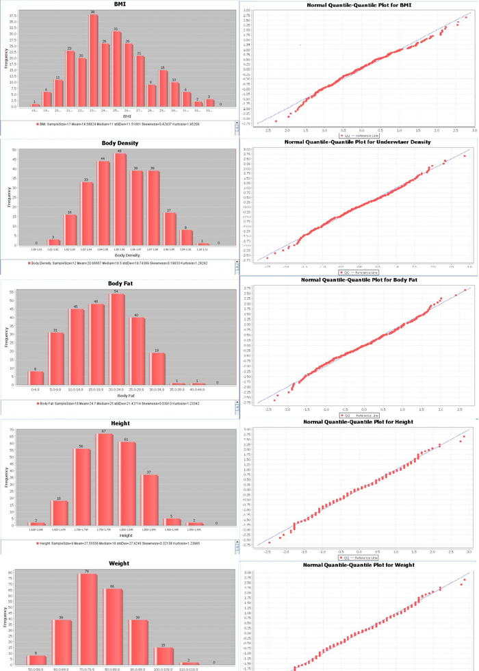
Exploratory data analyses (EDA)

Before we run any quantitative tests, let’s examine what these variables look like in graphical form. Keep an eye out for which variables appear to follow a normal distribution.

Quantitative Data Analyses (QDA)

In this section, we will be testing the BMI variable for normality, although the same analysis can be carried for the other variables. As the name goodness-of-fit implies, we first need to create a normal model to compare to. We will use the sample mean (25.18643319) and standard deviation (3.146481308) as the parameters of the normal distribution.

The next few steps will use the SOCR Distributions Applet (see Distribution Activities). Open the applet in a java-enabled browser.

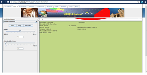
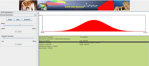
Enter in the values for the mean and standard deviation, then drag the graph down to see your full distribution.

To run a goodness of fit test, we will need to create a set of bins to compare between the real distribution and the expected normal one. For simplicity’s sake, we will use a 16 bins of bin-size 1 beginning with BMI=18 and ending with BMI=34. To find the frequency of results in each bin from the normal distribution, click on the edges of the bin size (try to be as accurate as possible) on the normal distribution applet. The example shown alternatively, use the normal CDF function.

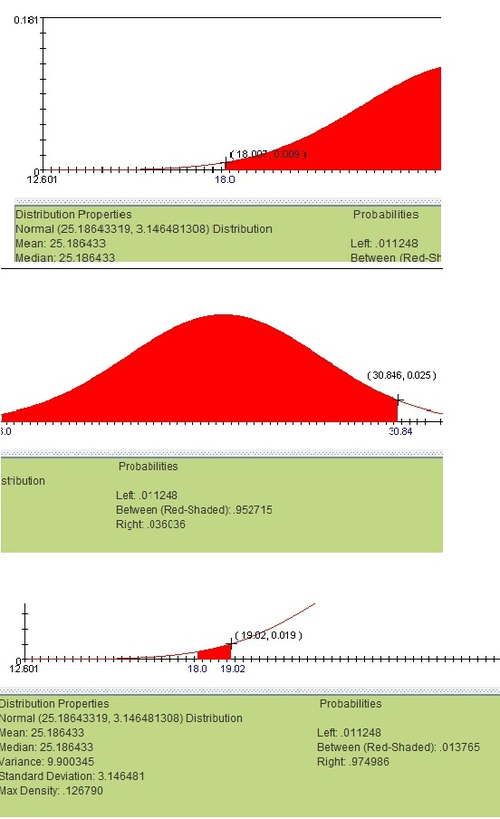
After calculating the probability of each bin, multiply each of these probabilities by the total number of cases (in this case, 248). Now we can place these calculated frequencies next to the frequencies from the observed distribution (the observed frequencies were found by plain counting):

Bin(Simplified)	Bin(Actual)	Normal_Probability	EstimatedNormalFrequency	ObservedFrequency
18-19	18.000-18.999	0.013454035	3.39041682	1
19-20	19.000-19.999	0.025001757	6.300442764	6
20-21	20.000-20.999	0.042032155	10.59210306	11
21-22	21.000-21.999	0.06392769	16.10977788	23
22-23	22.000-22.999	0.087962245	22.16648574	20
23-24	23.000-23.999	0.109497598	27.5933947	38
24-25	24.000-24.999	0.123313845	31.07508894	26
25-26	25.000-25.999	0.125638222	31.66083194	31
26-27	26.000-26.999	0.115806485	29.18323422	26
27-28	27.000-27.999	0.096570457	24.33575516	21
28-29	28.000-28.999	0.072854419	18.35931359	9
29-30	29.000-29.999	0.049724263	12.53051428	15
30-31	30.000-30.999	0.030702836	7.737114672	10
31-32	31.000-31.999	0.017150734	4.321984968	6
32-33	32.000-32.999	0.008667207	2.184136164	2
33-34	33.000-33.999	0.00396249	0.99854748	3

It might be useful to see how this hypothetical expected data matches up with our actual results graphically. Note the differences between the two data sets in the Quantile-Quantile Charts (ignore the stacked shape of the normal estimation, which is due to binning the data). Note that the line is a better fit in the latter case).

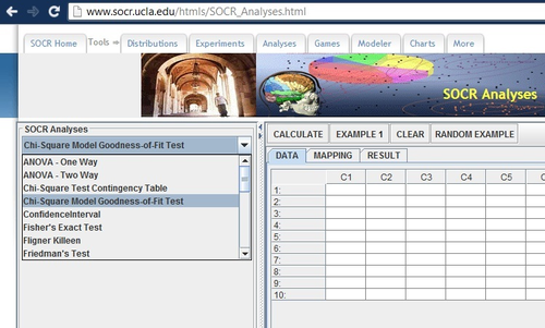
With these values now settled, we can begin the Chi-square analysis. Open up the SOCR Analyses Applet in a Java-enabled browser, and then select the Chi-square Goodness of Fit in the pull-down menu on the left:

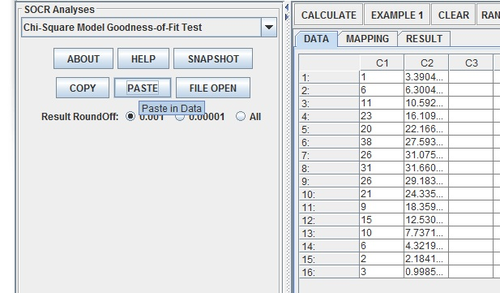
Next, enter the data into two columns using the Paste button.

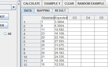
Name the two columns Observed (for the actual results) and Expected (for the normal model estimates).

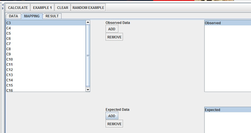
Click on the Mapping tab and add observed and expected into the correct bins.

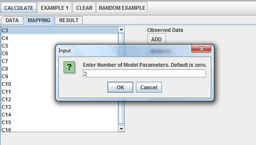
Click the Calculate Button. A window should pop up asking about the number of parameters. Recall that the normal distribution is defined by two parameters—mean and standard deviation. Enter “2” and press “OK”.

The results page should come up with the following text:

Observed Data = Observed

Expected Data = Expected

Chi-Square Goodness of Fit Results:

Total Counts = 16

Number of Parameters = 2

Chi-Square Goodness of Fit Results:

********** Chi-Square Statistic is: 21.044 *********

********** Chi-Square Degrees of Freedom is: 16 - 2 - 1 = 13 *********

********** Chi-Square p-value is: .072 *********

Based on α = 0.05, there is not enough evidence to conclude that the BMI data distribution does not fit a normal distribution. However, it is worth noting that it does come very close. This understanding of a distribution is very important to health officials; for example, it helps creates the charts that doctors national-wide use to understand. In addition, a deviation from that distribution can be used to chart changes in the overall health of the nation (Penman, 2006).

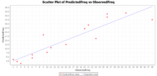
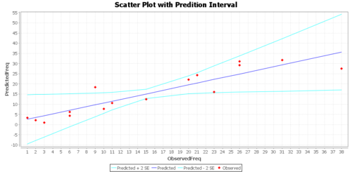
Finally, we can explore the correlation between the observed frequencies and the prediction-model values (predicted frequencies) of the BMI data within each of the 16 bins. If there is a good agreement (e.g., high correlation) this would indicate that the normal distribution model fits well the observed data (BMI frequencies).

Copy and paste the 2 column data (observed and predicted frequencies) into the Simple Linear Regression applet of [http://socr.ucla.edu/htmls/SOCR_Analyses.html SOCR Analysis.

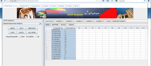
Map the predicted and observed frequencies to the Dependent and Independent variables (Mapping Tab).

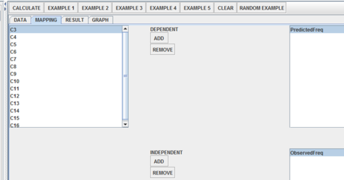
Click Calculate button to view the results. Regression Model:

PredictedFreq = 1.71070 + 0.8918062570205698 * ObservedFreq

Correlation(ObservedFreq, PredictedFreq) = .91394

R-Square = .83529

Intercept:

Parameter Estimate: 1.71070

Standard Error: 2.00468

T-Statistics: .85335

P-Value: .40783

Slope:

Parameter Estimate: .89181

Standard Error: .10584

T-Statistics: 8.42598

P-Value: .00000

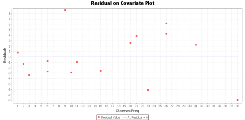
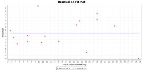
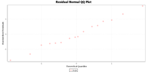
The Graphs tab includes a regression model plot, scatter plot with confidence/prediction limits, and various plots of the residuals.

Practice problems

• Try this method out on one of the other variables. See if it breaks from the normal distribution.
• Many biological measures are said to follow a normal distribution. Look under the data header “Biomedical Data” in the SOCR Free Datasets and check this claim out with one of the variables you are interested in.

See also

• SOCR Chi-Square Goodness-of-Fit Test

References

• K.W. Penrose, A.G. Nelson, A.G. Fisher, FACSM, Human Performance Research Center, Brigham Young University, Provo, Utah 84602 as listed in Medicine and Science in Sports and Exercise, vol. 17, no. 2, April 1985, p. 189.
• A.D. Penman and W.D. Johnson. University of Missisippi . Changing shape of the body mass index distribution curve in the population: implications for public health policy to reduce the prevalence of adult obesity." as listed in Preventing chronic disease, vol. 3, no. 2, 2006

---

---

Translate this page:

(default)	Deutsch	Español	Français	Italiano	Português	日本語	България	الامارات العربية المتحدة	Suomi	इस भाषा में	Norge
한국어	中文	繁体中文	Русский	Nederlands	Ελληνικά	Hrvatska	Česká republika	Danmark	Polska	România	Sverige