SOCR EduMaterials AnalysisActivities KruskalWallis

SOCR Analysis - Kruskal-Wallis Test Background

The Kruskal-Wallis Test is a generalization of the Two Independent Sample Wilcoxon Test. While the latter one test for two groups, the Kruskal-Wallis Test test multiple groups. Suppose there are k groups, the hypotheses are written as:

Null Hypothesis H_0: All of the k population distribution functions are identical.

Alternative Hypothesis H_A: At least one of the populations tends to yield larger observations than at least one of the other populations.

or

Alternative Hypothesis H_A: The k populations do not all have identical means. (k is the number of groups here.)

Rank sum is employed for hypotheses testing. Note that the sample size for each group do not have to be the same. Go to the Kruskal-Wallis Test Applet.

SOCR Analyses Example on the Kruskal-Wallis Test

The example we show here is from "Practical Nonparametric Statistics" by Conover, Second Edition, John Wiley & Sons, 1980. (Page 230)

Steps:

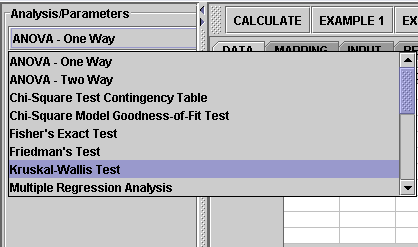
The data of this example has 4 groups: A, B, C and D. Click on "Kruskal-Wallis Test" from the conbo box in the left panel

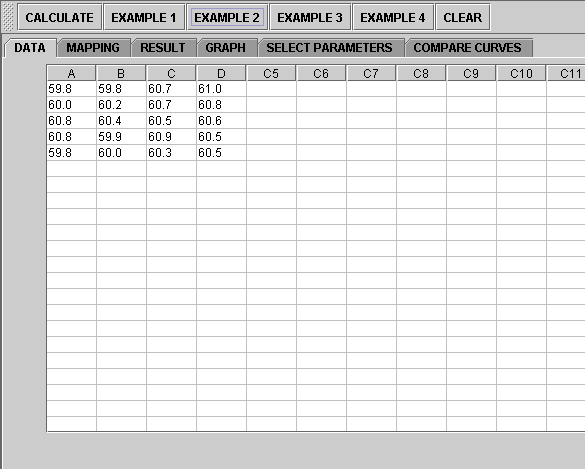
Click on "Example 2" button. than the "Data" button to see the data

The data need to be send to the computer for analysis

In the Kruskal-Wallis test, at least two groups need to be included. You can certainly include any two groups, any three groups, or all the available groups, etc., from the data set. The test will only analyze the groups selected. Therefore, you'll need to let the computer know what groups you're choosing. This is done in the "Mapping" panel. Click on the "Mapping" button to include the groups you want.

Next, click on the "Calculate" button

Now you're ready to see the results. Just click on the "Result" button.

Scroll down to see complete results.

If you'd like to include some other group(s) or remove the current groups and start over, simply go to the Mapping button and take the groups you want.

Note: if you happen to click on the "Clear" button in the middle of the procedure, all the data will be cleared out. Simply start over from step 1 and retrieve the data by click an EXAMPLE button.

Result Interpretation

• The Results tab ends with a summary like this:

Significance Level = 0.05

Degrees of Freedom = 16

Critical Value = 2.120

Test Statistic T = 7.487

S * S = 34.632

The test statistic that follows Student's t-distribution is:

|Ri/ni - Rj/nj| / sqrt(S * S * (N - 1 - T) / (N - k)) / sqrt(1/ni + 1/nj) (or identically)

$$\sqrt{{1\over n_i} + {1\over n_j}}\times {|{R_i\over n_i} - {R_j\over n_j}| \over ({S^2 (N - 1 - T) \over N - k})^{0.5}}$$

It is computed using T and S above. N is the total number of observations.

Notation: Ri -- Sum of ranks of group i; ni -- size of group i.

|Ri/ni - Rj/nj| 2.1199 * sqrt(24.9187) * sqrt(1/ni + 1/nj)

Group A vs. Group B: 3.1999 < 6.6928 (does not yield rejection of Ho)

Group A vs. Group C: 4.7000 < 6.6928 (does not yield rejection of Ho)

Group A vs. Group D: 5.7000 < 6.6928 (does not yield rejection of Ho)

Group B vs. Group C: 7.9 > 6.6928 (yields rejection of Ho)

Group B vs. Group D: 8.9 > 6.6928 (yields rejection of Ho)

Group C vs. Group D: 1.0 < 6.6928 (does not yield rejection of Ho)

Since Group B appears to have different mean ranks than group C and group D, the null hypothesis is rejected.

• These results include the critical value (2.120) and the value of the test statistics (T=7.487), which indicate that there is sufficient evidence (at \(\alpha=0.05\)) to reject the null hypothesis that the sample centers are equal.
• Also, the paired-group comparisons (accounting for multiple-testing) indicate the normal ranges of the rank differences between groups. For instance, Group B vs. Group C: 7.9 > 6.6928 indicates the range of normal rank differences between groups B and C.

References

• Conover, WJ (1980). Practical Nonparametric Statistics. John Wiley & Sons. Second Edition.

---

---

---

Translate this page:

(default)	Deutsch	Español	Français	Italiano	Português	日本語	България	الامارات العربية المتحدة	Suomi	इस भाषा में	Norge
한국어	中文	繁体中文	Русский	Nederlands	Ελληνικά	Hrvatska	Česká republika	Danmark	Polska	România	Sverige