SOCR EduMaterials AnalysisActivities LogisticRegression
Contents
[hide]SOCR Analysis Logistic Regression Analysis Activity
This SOCR Activity demonstrates the utilization of the SOCR Analyses package for statistical Computing. In particular, it shows how to use Simple Linear Regression and how to interpret the results.
Logistic Regression Background
Logistic Regression is a class of statistical analysis models and procedures, which takes one or more independent variable(s) and one binary dependent variable (a variable that can take on only two outcomes, e.g. “success” or “failure”), and models the relationship between them. The independent variables used in logistic regression may be continuous or categorical, depending on the situation. Note that the dependent variable follows a Bernoulli distribution with expected value equal to its probability of success.
The goal of the Logistic Regression computing procedure is to estimate the probability of success of the dependent variable given the observed independent variables. Its purpose will become clear as we start our explanation from the logistic function\[f(z)=\frac{e^{z}}{e^{z}+1}=\frac{1}{1+e^{-z}}\], where \(z=B_0+B_1 x_1+B_2 x_2+\cdots+B_n x_n\).
The logistic function has the characteristic that it can take input values ranging (-∞,∞) and the output value would always be between 0 and 1 inclusive. In the logistic function, the variable z models the “contribution” of each independent variable to the logistic function — a large coefficient (\(B_1, B_2, \cdots, B_n\)) usually denotes a profound impact of that particular independent variable on the probability of the outcome (the “success” of binary dependent variable), whereas a coefficient close to zero usually denotes a weak impact on the probability of the outcome. The coefficients are usually computed by some optimization technique, such as the method of maximum likelihood, which finds the coefficients that best fit the observed data.
Goals
In this activity, the students can learn about:
- Reading results of Logistic Regression;
- Making interpretation of the coefficients;
- Observing and interpreting various data and resulting plots
- Scatter plots of the dependent vs. independent variables
- Diagnostic plots such as the Residual on Fit plot
- Normal QQ plot, etc.
Data Input
Go to SOCR Analyses and select Logistic Regression from the drop-down list of SOCR analyses, in the left panel. There are two ways to enter data in the SOCR Logistic Regression applet:
- Click on the Example button on the top of the right panel.
- Paste your own data from a spreadsheet into SOCR Logistic Regression data table.
Example
We will demonstrate Logistic Regression with some SOCR built-in example. This example is based on a dataset from neuroimaging study of childhood-onset schizophrenia. The goals of the study were to identify associations and relationships between neuroimaging biomarkers and various subject demographics and traits.
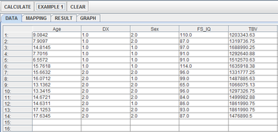
The data set describe a record of 14 subjects. There are five variables: Age for subject age, DX for subject diagnosis (Normals=1; Schizophrenia=2), Sex for subject gender (Male=1; female=2), FS_IQ for subject Intelligence Quotient (IQ), TBV for total brain volume (\(mm^3\)).
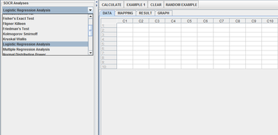
- As you start the SOCR Analyses Applet, click on "Logistic Regression" from the combo box in the left panel. Here's what the screen should look like.
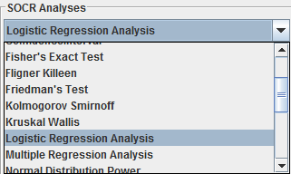
- The left part of the panel looks like this (make sure that the "Logistic Regression" is showing in the drop-down list of analyses, otherwise you won't be able to find the correct dataset and will not be able to reproduce the results!)
- In the SOCR Logistic analysis, there is one SOCR built-in example. Click on the "Example 1" button and next, click on the "Data" button in the right panel. You should see the data displayed in 5 columns: Age, DX, Sex, FS_IQ and TBV.
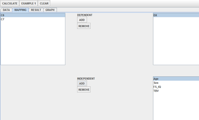
- Use column Age, Sex, FS_IQ and TBV as the regressors (independent variables) and column DX as the response (dependent variable). To tell the computer which variables are assigned to be the regressor and response, we have to do a "Mapping." This is done by clicking on the "Mapping" button first to get to the Mapping Panel, and then map the variables. For this Logistic Regression activity, there are two places the variables can be mapped to. The top part says DEPENDENT that you'll need to map the dependent variable you want here. Just click on ADD under DEPENDENT and that will do it. If you change your mind, you can click on REMOVE. Similar for the INDEPENDENT variable. Once you get the screen to look like the screenshot below, you're done with the Mapping step. (Note that, since the columns C6 through C16 do not have data and they are not used, just ignore them.)
- After we do the "Mapping" to assign variables, now we use the computer to calculate the regression results -- click on the "Calculate" button. Then select the "Result" panel to see the output. For each of the coefficients, Estimate stands for the estimated parameter value, followed by its Standard Error, T-Value and P-Value.
The text in the Result Panel summarizes the results of this Logistic regression analysis. At this point, you can think about how the dependent variable changes, on average, in response to changes of the independent variable. In this particular example, we see that TBV (total brain volume) has no influence on the subject diagnosis (as the coefficient associated with TBV is zero), whereas the subject’s sex contribute the most to his/her probability of being diagnosed with schizophrenia (because the absolute value of the coefficient associated with the variable Sex is the largest). Moreover, the regression model tells us that a 15 year old male subject with Age = 15, Sex = 1, FS_IQ = 90, TBV = 1400000(\(mm^3\)) would have a probability of 13.86% of being diagnosed with schizophrenia (the value of Z in the model after calculation).
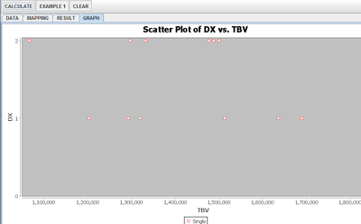
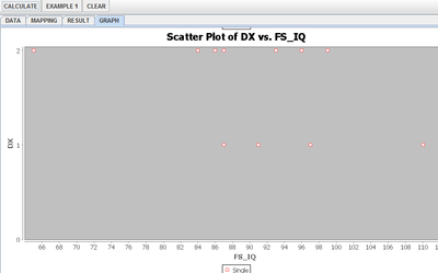
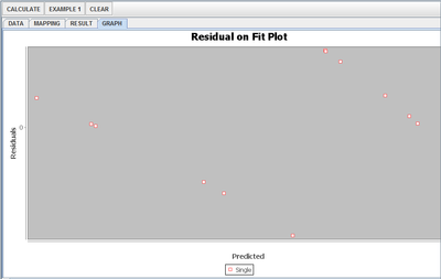
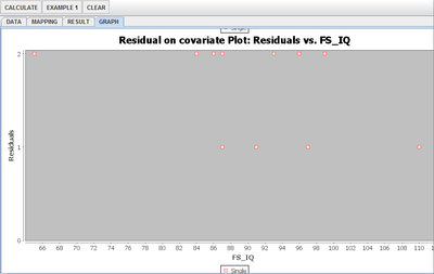
- If you'd like to see graphical component of this analysis, click on the "Graph" panel. You'll then see the graph panel that displays scatter plot, as well as diagnostic plots of "residual on fit", "Normal QQ" plots, etc. The plot titles indicate plot types.
Note: If you happen to click on the "Clear" button in the middle of the procedure, all the data will be cleared out. Simply start over from step 1 and click on an EXAMPLE button for the data you want.
Notes
- If one uses popular statistical software tools to perform logistic regression on any given dataset, the coefficients (betas) obtained may be different across several statistical platforms such as R, SPSS and SAS. However, in most cases, the area under ROC (Receiver-Operator Curve) should always be the same. As the SOCR Analysis Logistic Regression applet uses Newton-Raphson method to compute the beta coefficients, the result might be different from other statistical packages such as R, which uses another numerical method known as Fisher Scoring. Nonetheless, it can be checked that the areas under both ROCs match. Alternatively, one can check that the prediction error: \(\sum_{i=1}^n {(y_i-\hat{y}_i)^2}\) is the same in both cases.
- Data Close to Colinear error message indicates that some of the predictor variables are strongly linearly correlated. This may occur if the same variable is included repeatedly (as a column) in the data table, or when several different predictors are strongly correlated. Removing colinear variables, or changing some of these (e.g., log-transformation) prior to running the Logistic regression applet is required for correct estimation of effects (betas).
Translate this page: