SOCR EduMaterials AnalysisActivities PCA
SOCR Analysis - SOCR Principal Component Analysis Activity
This SOCR Activity demonstrates the utilization of the SOCR Analyses package for statistical Computing. In particular, it shows how to use Principal Component Analysis (PCA) and how to read the output results.
Principal Component Analysis Background
Principal Component Analysis is a mathematical procedure that transforms a number of possibly correlated variables into a fewer number of uncorrelated variables through a process known as orthogonal transformation. The resulting uncorrelated variables are called principal components. The first principal component accounts for as much of the variability in the data as possible, and each succeeding component accounts for the remaining variability. PCA is a useful statistical technique that has found application many fields, including computer networks and image processing, and is a powerful method for finding patterns high-dimension dataset.
Computational Details of Principal Component Analysis
1. We begin by obtaining a dataset that contains at least two dimensions (variables). The dataset can contain as many observations (dimensions) as possible.
2. After obtaining the original dataset, Step 2 is to normalize the observations for each variable. To do this, simply subtract the mean (average) from each observation in a given variable. For example, let X and Y be the two variables from the original dataset, with variable X containing observations \(X_1, X_2, X_3, \cdots , X_n \), and variable Y containing observations \(Y_1, Y_2, Y_3, \cdots , Y_n\). Let \(\bar{X}\) be the average of the n X observations, i.e., \(\bar{X} = \frac{X_1+ X_2+ X_3+ \cdots +X_n}{n}\), and similarly let \(\bar{Y}\) be the average of the Y observations. Then the normalized dataset would be:
- For variable X: \(X_1-\bar{X}, X_2-\bar{X}, X_3-\bar{X}, \cdots , X_n-\bar{X}\)
- For variable Y: \(Y_1-\bar{Y}, Y_2-\bar{Y}, Y_3-\bar{Y}, \cdots , Y_n-\bar{Y}\)
3. Calculate the covariance matrix between the variables of the normalized dataset.
4. Calculate the Eigenvalues and Eigenvectors of the covariance matrix. Note: The Eigenvectors must be normalized to have a length of 1.
5. Now we can choose our most “significant” principal component, which is simply the Eigenvector with the highest Eigenvalue. The Eigenvector corresponding to the second highest Eigenvalue will give us the next “significant” Eigenvector.
What do we mean by “significant”?
The principal components (i.e., Eigenvectors) are significant in the sense that they capture the most variability in the original dataset. Thus if we only take the first n Eigenvectors out of a dataset of dimension m, we’ve essentially compressed the dataset without losing too much information – and this is the fundamental idea behind Principal Component Analysis.
Goals
In this activity, the students can learn about:
- Inputting data in the correct formats;
- Reading results of Principal Component Analysis;
- Making interpretation of the resulting transformed data;
SOCR Principal Component Analysis Data Input
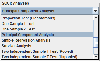
Go to SOCR Analyses and select Principal Component Analysis applet from the drop-down list of SOCR analyses, in the left panel. There are two ways to enter data in the SOCR Principal Component Analysis applet:
- Click on the Example button on the top of the right panel.
- Paste your own data from a spreadsheet into SOCR Principal Component Analysis data table.
SOCR Principal Component Analysis Example
We will demonstrate Principal Component Analysis with with some SOCR built-in example. This example is based on a dataset from the statistical program "R." For more information of the R program, please see CRAN Home Page. The dataset used here is "road" under R's "MASS" library. The dataset describes road accident deaths in US States. There are 6 variables: deaths for number of death, drivers for number of drivers (in 10,000s), popden for population density in people per square mile, rural for length of rural roads, in 1000s of miles, temp for average daily maximum temperature in January, fuel for fuel consumption in 10,000,000 US gallons per year.
As you start the SOCR Analyses Applet, click on "Principal Component Analysis " from the combo box in the left panel. Here's what the screen should look like.
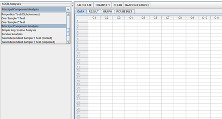
- The left part of the panel looks like this (make sure that the "Principal Component Analysis " is showing in the drop-down list of analyses, otherwise you won't be able to find the correct dataset and will not be able to reproduce the results!)
- In the SOCR PCA analysis, there is one SOCR built-in example. Click on the "Example 1" button and next, click on the "Data" button in the right panel. You should see the data displayed in 6 columns: deaths, drivers, popden, rural, temp, fuel.
- After opening the text file, the screen should look like this:
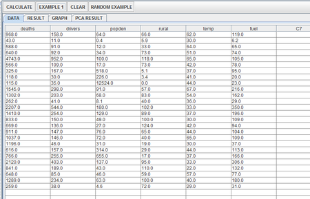
- As displayed, there are 26 observations for each of the 6 variables. After inputting the data, we now use the applet to produce the resulting principal components (including eigenvalues and eigenvectors calculated from the covariance matrix)
- Click on the "Calculate" button. At this point, a dialogue box will pop up and ask the user to select the variables used in this PCA analysis. By default (that is, if the user clicks “Yes”), then all 6 variables would be used in this analysis. If, however, the user only wants to use some of the variables above (e.g. drivers and popden only) and clicks “No”, then another dialogue box would pop up and prompt the user to input the column number of the desired variables, separated by commas:
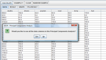
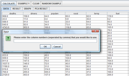
- Here we assume the user clicked on “Yes” and thus use all 6 variables for our PCA analysis. Click on the result panel, and it will look like this:
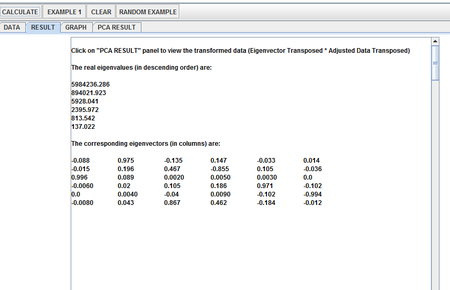
- To view the transformed data (in terms of the two principal axis), click on the Graph panel. In addition, a Scree Plot of eigenvalues (in descending order , computed from the covariance matrix) is also included:
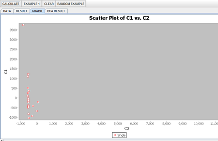
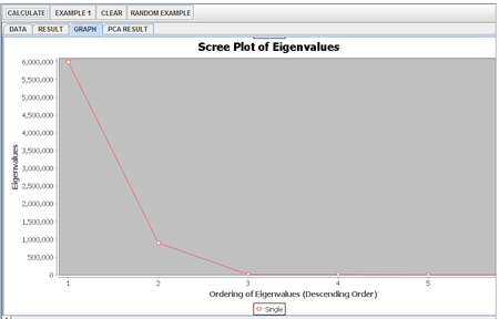
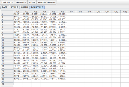
- Finally, the user can click on PCA Result panel to view the transformed data (computed as Eigenvector Transposed * Adjusted Data Transposed) in terms of the principal axis (note: each column corresponds to the original columns):
- Note: If you happen to click on the "Clear" button in the middle of the procedure, all the data will be cleared out. Simply start over from step 1 and click on an EXAMPLE button for the data you want.
Translate this page: