Difference between revisions of "SOCR EduMaterials AnalysisActivities ANOVA 2"
| (22 intermediate revisions by 2 users not shown) | |||
| Line 1: | Line 1: | ||
| − | + | ==[[SOCR_EduMaterials_AnalysesActivities | SOCR Analyses]] Example on Two-Way Analysis of Variance== | |
| + | === Background=== | ||
| + | [[AP_Statistics_Curriculum_2007_ANOVA_2Way | The 2-Way Analysis of Variance (ANOVA)]] is a statistical technique for analyzing study designs with one numerical outcome (response/dependent) variable and two categorical explanatory (predictor/independent) variables. For instance, in a completely randomized design we want to compare the response/outcome of a test by various subject-demographics (e.g., age, gender, disease severity, etc.) Subjects are grouped by one demographic-factor and then randomly assigned one treatment-factor (hence two-way!) | ||
| − | ''' | + | The methodological details about the 2-Way ANOVA may be found at [http://mathworld.wolfram.com/ANOVA.html Wolfram Research], [http://en.wikipedia.org/wiki/Analysis_of_variance Wikipedia] and [http://www.google.com/search?hl=en&q=two-way+ANOVA&btnG=Search elsewhere]. A motivational example demonstrating the need and utilization of 2-Way designs and analyses [http://www.uwsp.edu/psych/stat/13/anova-2w.htm can be found here]. |
| + | |||
| + | 2-way ANOVA is based on decomposing the variance of the response/dependent variable (total sum of squares) into '''within''' and '''between''' sum of squares. Sum of Squares '''between''' is then itself partitioned by intervention (blocking and interaction). | ||
| + | |||
| + | Typical hypotheses being tested in 2-way ANOVA are: | ||
| + | * Presense of significant main effects (within each of the 2 factors); | ||
| + | * Presense of an interaction between the two factors. | ||
| + | |||
| + | ===Examples=== | ||
| + | |||
| + | Go to the [http://www.socr.ucla.edu/htmls/ana/ANOVA2Way_Analysis.html SOCR 2-Way ANOVA Applet]. This really simple SOCR built-in example, '''EXAMPLE 1''' uses a dataset from [http://www.amazon.ca/Introduction-Computational-Statistics-Regression-Analysis/dp/0134548108 An Introduction to Computational Statistics: Regression Analyses" by Robert Jennrich, Prentice Hall, 1995 (Page 207)]. The data are about the time taken for coins to drop into different water fountain. Here, the dependent variable is time taken. And the two independent variables are: '''I''' for coin type, where "'''1'''" denotes for quarters and "'''2'''" for dimes; '''J''' for three different fountains. Our interest is to see if time is significantly related to these two independent factors. This example demonstrates a general two-way additive ANOVA model. | ||
| + | |||
| + | Here are the steps of the activities: | ||
| − | |||
| − | [[Image: | + | * Click on "'''Anova Two Way'''" at the '''left''' panel's combo box. |
| + | |||
| + | |||
| + | <center>[[Image:SOCR_AnalysisActivities_AnovaTwoWay_Chu_051707_Fig1.gif|700px]]</center> | ||
| + | |||
| + | |||
| + | <center>[[Image:SOCR_AnalysisActivities_AnovaTwoWay_Chu_051707_Fig2.gif|450px]]</center> | ||
| + | |||
| + | |||
| + | On the '''right''' panel, first click on "'''EXAMPLE 1'''" and next click on "'''Data'''" to retreive the demonstrating example. The column '''X''' is '''time''', the response variable, which is treated as a quantitative variable. The columns '''I''' and '''J''' are the independent variables. | ||
| + | |||
| + | |||
| + | <center>[[Image:SOCR_AnalysisActivities_AnovaTwoWay_Chu_051707_Fig1B.gif|700px]]</center> | ||
| + | |||
| + | |||
| + | * Click on the "'''Mapping'''" button to get to the "Mapping" panel. Click on "'''ADD'''" under '''Dependent''' to add '''X''', and click on "'''ADD'''" under Independent to add '''I''' and '''J'''. | ||
| + | |||
| + | |||
| + | <center>[[Image:SOCR_AnalysisActivities_AnovaTwoWay_Chu_051707_Fig3.gif|700px]]</center> | ||
| + | |||
| + | |||
| + | * Next, click on "'''Calculate'''" to let the computer do the calculation. Then click on "'''Result'''" to see the results. | ||
| + | |||
| + | |||
| + | <center>[[Image:SOCR_AnalysisActivities_AnovaTwoWay_Chu_051707_Fig3A.gif|700px]]</center> | ||
| + | |||
| + | |||
| + | * Plots are available for vewing and checking regression dignostics. Click on "'''Graph'''" to see plots. | ||
| + | |||
| + | |||
| + | |||
| + | <center>[[Image:SOCR_AnalysisActivities_AnovaTwoWay_Chu_051707_Fig4.gif|700px]]</center> | ||
| + | |||
| + | |||
| + | <center>[[Image:SOCR_AnalysisActivities_AnovaTwoWay_Chu_051707_Fig5.gif|700px]]</center> | ||
| − | + | <center>[[Image:SOCR_AnalysisActivities_AnovaTwoWay_Chu_051707_Fig6.gif|700px]]</center> | |
| − | [[Image: | + | <center>[[Image:SOCR_AnalysisActivities_AnovaTwoWay_Chu_051707_Fig7.gif|700px]]</center> |
| + | <center>[[Image:SOCR_AnalysisActivities_AnovaTwoWay_Chu_051707_Fig8.gif|700px]]</center> | ||
| − | |||
| − | [[Image: | + | <center>[[Image:SOCR_AnalysisActivities_AnovaTwoWay_Chu_051707_Fig9.gif|700px]]</center> |
| + | ===Technical Notes=== | ||
| + | ====SOCR vs. R and SAS 2-Way ANOVA==== | ||
| + | SOCR 2-Way ANOVA handles repeated measures and some of the default examples cover this situation (e.g., Example 2). | ||
| + | There is a difference between the [http://www.r-project.org R]-based and [http://www.sas.com/ SAS]-based approaches to repeated measures. In SOCR 2-Way ANOVA, we follow the SAS model and apply the ''dummy variable method'' described in [http://www.amazon.ca/Introduction-Computational-Statistics-Regression-Analysis/dp/0134548108 Jennrich's book]. Thus, the SOCR results format is the same as the output of SAS, in terms of degrees of freedom, sum of squares, etc. R's output is a little different from SAS's, and therefore it's not the same as the results reported by SOCR. In R, the order of the two factors (J and K) matters in the input. That is, if you put factor J first or K first, then the 2-way Anova results will be different. When the second factor is evaluated, the first one is considered fixed in R. | ||
| − | + | ===See also=== | |
| + | * [[SOCR_Activity_ANOVA_SnailsSexualDimorphism| SOCR ANOVA Snails Sexual Dimorphism Activity]] | ||
| − | + | {{translate|pageName=http://wiki.stat.ucla.edu/socr/index.php?title=SOCR_EduMaterials_AnalysisActivities_ANOVA_2}} | |
Latest revision as of 18:55, 28 November 2012
Contents
SOCR Analyses Example on Two-Way Analysis of Variance
Background
The 2-Way Analysis of Variance (ANOVA) is a statistical technique for analyzing study designs with one numerical outcome (response/dependent) variable and two categorical explanatory (predictor/independent) variables. For instance, in a completely randomized design we want to compare the response/outcome of a test by various subject-demographics (e.g., age, gender, disease severity, etc.) Subjects are grouped by one demographic-factor and then randomly assigned one treatment-factor (hence two-way!)
The methodological details about the 2-Way ANOVA may be found at Wolfram Research, Wikipedia and elsewhere. A motivational example demonstrating the need and utilization of 2-Way designs and analyses can be found here.
2-way ANOVA is based on decomposing the variance of the response/dependent variable (total sum of squares) into within and between sum of squares. Sum of Squares between is then itself partitioned by intervention (blocking and interaction).
Typical hypotheses being tested in 2-way ANOVA are:
- Presense of significant main effects (within each of the 2 factors);
- Presense of an interaction between the two factors.
Examples
Go to the SOCR 2-Way ANOVA Applet. This really simple SOCR built-in example, EXAMPLE 1 uses a dataset from An Introduction to Computational Statistics: Regression Analyses" by Robert Jennrich, Prentice Hall, 1995 (Page 207). The data are about the time taken for coins to drop into different water fountain. Here, the dependent variable is time taken. And the two independent variables are: I for coin type, where "1" denotes for quarters and "2" for dimes; J for three different fountains. Our interest is to see if time is significantly related to these two independent factors. This example demonstrates a general two-way additive ANOVA model.
Here are the steps of the activities:
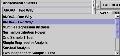
- Click on "Anova Two Way" at the left panel's combo box.


On the right panel, first click on "EXAMPLE 1" and next click on "Data" to retreive the demonstrating example. The column X is time, the response variable, which is treated as a quantitative variable. The columns I and J are the independent variables.

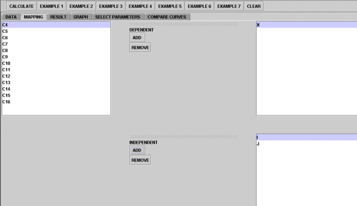
- Click on the "Mapping" button to get to the "Mapping" panel. Click on "ADD" under Dependent to add X, and click on "ADD" under Independent to add I and J.

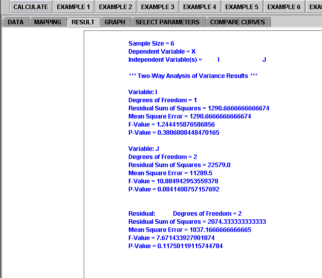
- Next, click on "Calculate" to let the computer do the calculation. Then click on "Result" to see the results.

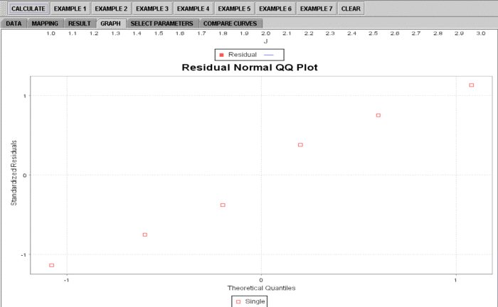
- Plots are available for vewing and checking regression dignostics. Click on "Graph" to see plots.


Technical Notes
SOCR vs. R and SAS 2-Way ANOVA
SOCR 2-Way ANOVA handles repeated measures and some of the default examples cover this situation (e.g., Example 2). There is a difference between the R-based and SAS-based approaches to repeated measures. In SOCR 2-Way ANOVA, we follow the SAS model and apply the dummy variable method described in Jennrich's book. Thus, the SOCR results format is the same as the output of SAS, in terms of degrees of freedom, sum of squares, etc. R's output is a little different from SAS's, and therefore it's not the same as the results reported by SOCR. In R, the order of the two factors (J and K) matters in the input. That is, if you put factor J first or K first, then the 2-way Anova results will be different. When the second factor is evaluated, the first one is considered fixed in R.
See also
Translate this page: