Difference between revisions of "SMHS SurvivalAnalysis"
(→References) |
|||
| Line 172: | Line 172: | ||
===References=== | ===References=== | ||
| − | + | ||
| − | * [http:// | + | * [http://en.wikipedia.org/wiki/Survival_analysis Survival Analysis Wikipedia] |
| − | * [http:// | + | *[http://en.wikipedia.org/wiki/Hazard_ratio Hazard Ratio Wikipedia] |
<hr> | <hr> | ||
Revision as of 12:31, 29 August 2014
Contents
Scientific Methods for Health Sciences - Survival Analysis
Overview
Survival analysis is statistical methods for analyzing longitudinal data on the occurrence of events. Events may include death, injury, onset of illness, recovery from illness (binary variables) or transition above or below the clinical threshold of a meaningful continuous variable (e.g. CD4 counts). Typically, survival analysis accommodates data from randomized clinical trial or cohort study designs. In this section, we will present a general introduction to survival analysis including terminology and data structure, survival/hazard functions, parametric versus semi-parametric regression techniques and introduction to (non-parametric) Kaplan-Meier methods. Code examples are also included showing the applications survival analysis in practical studies.
Motivation
Studies in the field of public health often involve questions like “What is the proportion of a population which will survive past time t?” “What is the expected rate of death in study participants, or the population”? “How do particular circumstances increase or decrease the probability of survival?” To answer questions like this, we would need to define the term of lifetime and model the time to event data. In cases like this, death or failure is considered as an event in survival analysis of time duration to until one or more events happen.
Theory
Hazard Ratios
Hazard is the slope of the survival curve — a measure of how rapidly critical events occur (e.g., subjects are dying).
- The hazard ratio compares two treatments. If the hazard ratio is 2.0, then the rate of deaths in one treatment group is twice the rate in the other group.
- The hazard ratio is not computed at any one time point, but is computed from all the data in the survival curve.
- Since there is only one hazard ratio reported, it can only be interpreted if you assume that the population hazard ratio is consistent over time, and that any differences are due to random sampling. This is called the assumption of proportional hazards.
- If the hazard ratio is not consistent over time, the value reported for the hazard ratio may not be useful. If two survival curves cross, the hazard ratios are certainly not consistent (unless they cross at late time points, when there are few subjects still being followed so there is a lot of uncertainty in the true position of the survival curves).
- The hazard ratio is not directly related to the ratio of median survival times. A hazard ratio of 2.0 does not mean that the median survival time is doubled (or halved). A hazard ratio of 2.0 means a patient in one treatment group who has not died (or progressed, or whatever end point is tracked) at a certain time point has twice the probability of having died (or progressed...) by the next time point compared to a patient in the other treatment group.
- Hazard ratios, and their confidence intervals, may be computed using two methods, each reporting both the hazard ratio and its reciprocal. If people in group A die at twice the rate of people in group B (HR=2.0), then people in group B die at half the rate of people in group A (HR=0.5).
The LogRank and Mantel-Haenszel methods
Both, the LogRank and Mantel-Haenszel methods usually give nearly identical results, unless in situations when several subjects die at the same time or when the hazard ratio is far from 1.0.
- The Mantel-Haenszel method reports hazard ratios that are further from 1.0 (so the reported hazard ratio is too large when the hazard ratio is greater than 1.0, and too small when the hazard ratio is less than 1.0):
- (1) Compute the total variance, V;
- (2) Compute $K = \frac{O1 - E1}{V}$, where $O1$ - is the total observed number of events in group1, $E1$ is the total expected number of events in group1. You'd get the same value of $K$ if you used the other group;
- (3) The hazard ratio equals $e^K$;
- (4) The 95% confidence interval of the hazard ratio is: ($e^{K - \frac{1.96}{\sqrt{V}}}$, $e^{K + \frac{1.96}{\sqrt{V}}}$).
- The logrank method (referred to as O/E method) reports values that are closer to 1.0 than the true Hazard Ratio, especially when the hazard ratio is large or the sample size is large. When there are ties, both methods are less accurate. The logrank methods tend to report hazard ratios that are even closer to 1.0 (so the reported hazard ratio is too small when the hazard ratio is greater than 1.0, and too large when the hazard ratio is less than 1.0):
- (1) As part of the Kaplan-Meier calculations, compute the number of observed events (deaths, usually) in each group ($O_a$ and $O_b$), and the number of expected events assuming a null hypothesis of no difference in survival ($E_a$ and $E_b$);
- (2) The hazard ratio then is: $HR= \frac{\frac{O_a}{O_a}}{\frac{O_b}{E_b}}$;
- (3) The standard error of the natural logarithm of the hazard ratio is: $\sqrt{\frac{1}{E_a} + \frac{1}{E_b}}$;
- (4) The lower and upper limits of the 95% confidence interval of the hazard ratio are: $e^{\frac{O_a-E_a}{V} \pm 1.96 \sqrt{\frac{1}{E_a} + \frac{1}{E_b}}}$.
Survival analysis goals
- Estimate time-to-event for a group of individuals, such as time until second heart-attack for a group of MI patients;
- To compare time-to-event between two or more groups, such as treated vs. placebo Myocardial infarction (MI) patients in a randomized controlled trial;
- To assess the relationship of co-variables to time-to-event, such as: does weight, insulin resistance, or cholesterol influence survival time of MI patients?
Terminology
- Time-to-event: The time from entry into a study until a subject has a particular outcome
- Censoring: Subjects are said to be censored if they are lost to follow up or drop out of the study, or if the study ends before they die or have another outcome of interest. They are (censored) counted as alive or disease-free for the time they were enrolled in the study. If dropout is related to both outcome and treatment, dropouts may bias the results.
- Two-variable outcome: time variable: $t_i$ = time of last disease-free observation or time at event; censoring variable: $c_i=1$ if had the event; $c_i =0$ no event by time $t_i$.
- Right Censoring ($T>t$): Common examples: termination of the study; death due to a cause that is not the event of interest; loss to follow-up. We know that subject survived at least to time $t$.
- Example: Suppose subject 1 is enrolled at day 55 and dies on day 76, subject 2 enrolls at day 87 and dies at day 102, subject 3 enrolls at day 75 but is lost (censored) by day 81, and subject 4 enrolls in day 99 and dies at day 111. The Figure below shows these data graphically. Note of varying start times. This figure is generated using the SOCR Y Interval Chart.

- The next Figure shows a plot of every subject's time since their baseline time collection (right censoring).

Survival distributions
- $T_i$, the event time for an individual, is a random variable having certain probability distribution;
- Different models for survival data are distinguished by different choice of distribution for the variable $T_i$;
- Parametric survival analysis is based on Waiting Time distributions (e.g., exponential probability distribution);
- Assume that times-to-event for individuals in a dataset follow a continuous probability distribution (for which we may have an analytic mathematical representation or not). For all possible times $T_i$ after baseline, there is a certain probability that an individual will have an event at exactly time $T_i$. For example, human beings have a certain probability of dying at ages 1, 26, 86, 100, denoted by $P(T=1)$, $P(T=26)$, $P(T=86)$, $P(T=100)$, respectively, and these probabilities are obviously vastly different from one another;
- Probability density function f(t): In the case of human longevity, $T_i$ is unlikely to follow a unimodal normal distribution, because the probability of death is not highest in the middle ages, but at the beginning and end of life (bimodal?). The probability of the failure time occurring at exactly time $t$ (out of the whole range of possible $t$’s) is: $f(t)=log_{∆t→0}\frac{P(t≤T<t+∆t)}{∆t}$.
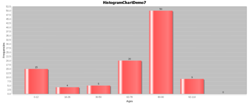
- Example: Suppose we have the following hypothetical data (Figure below). People have a high chance of dying in their 70’s and 80’s, but they have a smaller chance of dying in their 90’s and 100’s, because few people make it long enough to die at these ages.

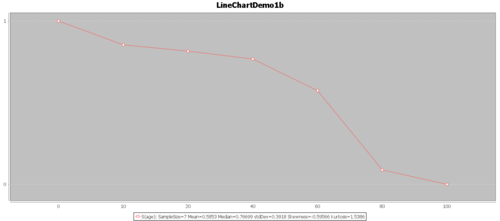
- The Survival function, $S(t)=1-F(t)$: The goal of survival analysis is to estimate and compare survival experiences of different groups. Survival experience is described by the cumulative survival function: $S(t)=1-P(T≤t)=1-F(t)$, where $F(t)$ is the CDF of $f(t)$. The Figure below shows the cumulative survival for the same hypothetical data, plotted as cumulative distribution rather than density.

Try to use real-data and the SOCR Survival Analysis and the SOCR Survival Java Applet to generate a similar plot.
- Hazard function represents the probability that if you survive to $t$, you will succumb to the event in the next instant.
$$h(t)=log_{∆t→0} \frac{P(t≤T<t+∆t|T≥t)}{∆t}.$$
- The Hazard function may also be expressed in terms of density and survival: $h(t)=f(t)/S(t)$. This is because of the Bayesian rule:
$$h(t)dt = P(t≤T<t+dt|T≥t)=\frac{P(t≤T<t+dt \cap T≥t)}{P(T≥t)} =\frac{P(t≤T<t+dt){}P(T≥t)} =\frac{f(t)dt}{S(t)}.$$
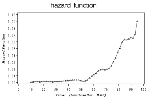
- The Figure below illustrates an example plot of a hazard function depicting the hazard rate as an instantaneous incidence rate.

- Examples
- For uncensored data, the following failure time are observed for n=10 subjects. For convenience, the failure times have been ordered. Calculate $\hat{S}(20)$.
| i | 1 | 2 | 3 | 4 | 5 | 6 | 7 | 8 | 9 | 10 |
|---|---|---|---|---|---|---|---|---|---|---|
| $T_i$ | 2 | 5 | 8 | 12 | 15 | 21 | 25 | 29 | 30 | 34 |
$$\hat{S}(20)=0.5.$$
- For censored data, suppose instead the observed data were:
| i | 1 | 2 | 3 | 4 | 5 | 6 | 7 | 8 | 9 | 10 |
|---|---|---|---|---|---|---|---|---|---|---|
| $X_i$ | 2 | 5 | 8 | 12 | 15 | 21 | 25 | 29 | 30 | 34 |
| $∆_i$ | 1 | 0 | 1 | 0 | 1 | 0 | 1 | 0 | 1 | 0 |
$$\hat{h}(2)=0.1; \hat{h}(8)=0.125; \hat{h}(15)=0.166.$$
- Cumulative Hazard function is defined as $Λ(t)=\int_0^t{h(u)du}$. There is an important connection between cumulative hazard and survival: $S(t)=e^{-Λ(t)}$, although, the cumulative hazard function may be hard to interpret. Note that $e^{-a} \approx 1-a$ for small $a$. Thus, we have $e^{-λ(u)} \approx 1-λ(u)$, taking product between 0 and t on both sides, we have $e^{-Λ(t)}=\prod_{u \in (0,t]}{1-λ(u)du}$.
- Properties:
- (1) $Λ(t)≥0$;
- (2) $log_{t→∞}{Λ(t)}=\infty$;
- (3) $Λ(0)=0$.
- Hazard vs. density example: at birth, each person has a certain probability of dying at any age; that’s the probability density (cf. marginal probability). For example: a girl born today may have a 2% chance of dying at the age of 80 years. However, if a person survives for a while, the probabilities of prospective survival change (cf. conditional probability). For example, a woman who is 79 today may have a 6% chance of dying at the age of 80. The figure bellow gives a set of possible probability density, failure, survival and hazard function. $F(t)$=cumulative failure=$1-e^{-t^1.7}$; $f(t)$=density function=$1.7 t^{0.7} e^{-t^{1.7}}$; $S(t)$=cumulative survival=$e^{-t^{1.7}}$; $h(t)$=hazard function=$1.7t^{0.7}$.

Common density functions describing survival probability
- Exponential (hazard is constant over time, simplest model!): constant hazard function $h(t)=h$; exponential density functions: $P(T=t)=f(t)=he^{-ht}$; survival function $P(T>t)=S(t)=\int_t^{\infty} {he^{-hu} du}=-e^{-hu} |_t^{\infty}=e^{-ht}$.
- Example: $h(t)=0.1$ cases/person-year; Then
- the probability of developing disease at year 10 is: $P(t=10)=0.01e^{-0.1*10}=0.01e^{-0.1}=0.009$;
- the probability of surviving past year 10 is: $S(t)=e^{-0.01t}=90.5%$;
- the cumulative risk through year 10 is 9.5%.
- Weibull (hazard function is increasing or decreasing over time)
Mathematical formulation/relations
- Hazard from density and survival: $h(t)=\frac{f(t)}{S(t)}$
- Survival from density: $S(t)=\int_t^{\infty} {f(u)du}$
- Density from survival: $f(t)=-\frac{dS(t)}{dt}=S(t)h(t)$
- Density from hazard: $f(t)=h(t) e^(-\int_0^t {h(u)du}$
- Survival from hazard: $S(t)=e^(-\int_0^t {h(u)du}$
- Hazard from survival: $h(t)=-\frac{d}{dt} \ln{S(t)}$
- Cumulative hazard from survival: $Λ(t)=-\log{S(t)}$
- Life expectancy (mean survival time): $E[T]=\int_0^{\infty} {tf(t)dt}=\int_0^{\infty} {S(t)}$, which is the area under the survival curve
- Restricted mean lifetime: $E[T∧L]=\int_0^L {S(t)dt}$
- Mean residual lifetime: $m(t_0)=E[T-t_0|T>t_0]=\int_{t_0}^{\infty}{\frac{(t-t_0)f(t)dt}{S(t_0)}}=\int_{t_0}^{\infty} {\frac{S(t)dt}{S(t_0)}}$, set $t_0=0$ to obtain E[T].
Hazard function models
- Parametric multivariate regression techniques: model the underlying hazard/survival function; assume that the dependent variable (time-to-event) takes on some known distribution, such as Weibull, exponential, or lognormal; estimates parameters of these distributions (e.g., baseline hazard function); estimates covariate-adjusted hazard ratios (a hazard ratio is a ratio of hazard rates); many times we care more about comparing groups than about estimating absolute survival. The model of parametric regression: components include a baseline hazard function (which may change over time) and a linear function of a set of k fixed covariates that when exponentiated gives the relative risk.
- Exponential model assumes fixed baseline hazard that we can estimate: with exponential distribution, $S(t)=e^{-λt}$, model applied: $\log{h_i(t)}=μ+β_1 x_{i1}+⋯+β_k x_{ik}$;
- Weibull model models the baseline hazard as a function of time: two parameters of shape ($\gamma$) and scale ($λ$) must be estimated to describe the underlying hazard function over time. With Weibull distribution: $S(t)=e^{-λt^{\gamma}}$, model applied: $\log {h_i(t)}= μ+α\log{t}+β_1 x_{i1}+⋯+β_k x_{ik}$;
- Cox regression (semi-parametric): Cox models the effect of predictors and covariates on the hazard rate but leaves the baseline hazard rate unspecified; also called proportional hazards regression; does not assume knowledge of absolute risk; estimates relative rather than absolute risk.
- Components: a baseline hazard function that is left unspecified but must be positive (equal to the hazard when all covariates are 0); a linear function of a set of $k$ fixed covariates that is exponentiated (equal to the relative risk).
- $\log{h_i(t)}= \log{h_0 (t)}+β_1 x_{i1}+⋯+β_k x_{ik}$; $h_i (t)=h_0(t) e^{β_1 x_{i1}+⋯+β_k x_{ik}}$.
- The point is to compare the hazard rates of individuals who have different covariates: hence, called Proportional hazards: $HR=\frac{h_1 (t)}{h_2 (t)}=\frac{h_0 (t) e^{βx_1 }}{h_0 (t) e^{βx_2}}=e^{β(x_1-x_2)}$, hazard functions should be strictly parallel.
- Kaplan-Meier Estimates (non-parametric estimate of the survival function): no a priori math assumptions (either about the underlying hazard function or about proportional hazards); simply, the empirical probability of surviving past certain times in the sample (taking into account censoring); non-parametric estimate of the survival function; commonly used to describe survivorship of study population/s; commonly used to compare two study populations; intuitive graphical presentation.
- Limit of Kaplan-Meier: this approach is mainly descriptive, doesn’t control for covariates, requires categorical predictors and can’t accommodate time-dependent variables.
- With Kaplan-Meier: (for uncensored data) $\hat{S}(t)=\frac{1}{n}\sum_{i=1}^n{I(T_i>t)}$, where $I(A)=1$ if $A$ is true and 0 otherwise. (for censored data, calculated in censoring free subintervals). For example:
| i | 1 | 2 | 3 | 4 | 5 | 6 | 7 | 8 | 9 | 10 |
|---|---|---|---|---|---|---|---|---|---|---|
| $X_i$ | 2 | 5 | 8 | 12 | 15 | 21 | 25 | 29 | 30 | 34 |
| $∆_i$ | 1 | 0 | 1 | 0 | 1 | 0 | 1 | 0 | 1 | 0 |
To estimate $S(10)$: $S(10)=P(T>10)=P(T>10,T>8,T>5,T>2)=P(T>10│T>8)P(T>8│T>5)P(T>5│T>2)P(>2)=9/10*9/9*7/8*7/7=0.7875$. So, $\hat{S}_{KM}(10)=0.7875$. Example survival data (right-censored):
The product limit estimate: the probability of surviving in the entire year, taking into account censoring P= (4/5) (2/3) = 53%. Note that: (1) P > 40% (2/5) because the one drop-out survived at least a portion of the year; (2) P<60% (3/5) because we don’t know if the one drop-out would have survived until the end of the year.
Figure 6 Compare two groups. Use log-rank test to test the null hypothesis of no difference between survival functions of the two groups. USE SOCR APPLET to chart … Caution: Survival estimates can be unreliable toward the end of a study when there are small numbers of subjects at risk of having an event.
References
- SOCR Home page: http://www.socr.umich.edu
Translate this page: