Difference between revisions of "SMHS LinearModeling MLR VizModelCoeff"
(→Normality of residuals) |
(→Protocols for Rectifying Residual Plots Indicating Nonlinearity) |
||
| (6 intermediate revisions by one other user not shown) | |||
| Line 80: | Line 80: | ||
<center>[[Image:SMHS_LinearModeling_Fig20.png|500px]]</center> | <center>[[Image:SMHS_LinearModeling_Fig20.png|500px]]</center> | ||
| − | ===Protocols for | + | ===Protocols for Rectifying Residual Plots Indicating Nonlinearity=== |
Model may be excluding important fixed effects that interact with fixed effects already accounted for in the model. If new fixed effects are added, the pattern in the residual plot may disappear. | Model may be excluding important fixed effects that interact with fixed effects already accounted for in the model. If new fixed effects are added, the pattern in the residual plot may disappear. | ||
| − | + | *Variable transformation – Perform a nonlinear transformation of the response, e.g., log, or reciprocal transform. See this SOCR Activity<sup>5</sup>. | |
| − | + | *Perform a nonlinear transformation to explanatory variables. For instance, if Age is related to Weight in a U-shaped way (e.g., quadratic relation), then the model could include Age and Age<sup>2</sup> as predictors. | |
| − | + | *If residual plots include stripes, then there may be categorical variables playing role, which may necessitate alternative class of models, such as logistic or multinomial models. | |
| − | ===Lack of | + | ===Lack of Collinearity=== |
A pair of (linearly) correlated predictors are also called collinear. Suppose Age and Height are correlated (which is certainly to be expected!), then including both as predictors of Weight presents a collinearity problem. In the presence of significant variable collinearity, the interpretation of the model becomes challenging. Depending on which correlated predictors are included in the model, the fixed effects may (incorrectly) become significant or insignificant. Significant findings for these correlated or collinear fixed effects is difficult to interpret as there may be trading-off between the "explanatory power" of the pair of covariates. Multiple predictors that are very similar (linearly correlated) inhibit our ability to decide what plays a big role and what has only marginal impact on the response. | A pair of (linearly) correlated predictors are also called collinear. Suppose Age and Height are correlated (which is certainly to be expected!), then including both as predictors of Weight presents a collinearity problem. In the presence of significant variable collinearity, the interpretation of the model becomes challenging. Depending on which correlated predictors are included in the model, the fixed effects may (incorrectly) become significant or insignificant. Significant findings for these correlated or collinear fixed effects is difficult to interpret as there may be trading-off between the "explanatory power" of the pair of covariates. Multiple predictors that are very similar (linearly correlated) inhibit our ability to decide what plays a big role and what has only marginal impact on the response. | ||
| Line 148: | Line 148: | ||
The histogram (left) is relatively bell-shaped and the Q-Q normal probability plot (right) indicates the residuals are mostly on a straight line (suggesting errors (observed-predicted) are similar to a normal distribution). Thus, there is no strong evidence suggesting possible violation of the normality assumption. | The histogram (left) is relatively bell-shaped and the Q-Q normal probability plot (right) indicates the residuals are mostly on a straight line (suggesting errors (observed-predicted) are similar to a normal distribution). Thus, there is no strong evidence suggesting possible violation of the normality assumption. | ||
| − | + | ===Outliers (influential data points)=== | |
Data should not include extreme influential points, otherwise the linear model may be heavily biased. Outliers (influential data points) can drastically change the interpretation of model results and inference, similarly to variable collinearity. | Data should not include extreme influential points, otherwise the linear model may be heavily biased. Outliers (influential data points) can drastically change the interpretation of model results and inference, similarly to variable collinearity. | ||
| Line 191: | Line 191: | ||
Interpretation of large or a small DFbeta values is similarly "open" as the interpretation of p-values (case-specific). However, if the DFbeta value changes, the sign of the coefficient slope, then this data point is an outlier candidate (influential point) that needs special attention. Excluding that 1 point would change the interpretation of the model results. | Interpretation of large or a small DFbeta values is similarly "open" as the interpretation of p-values (case-specific). However, if the DFbeta value changes, the sign of the coefficient slope, then this data point is an outlier candidate (influential point) that needs special attention. Excluding that 1 point would change the interpretation of the model results. | ||
| − | For small to medium size (n) data, |DFbeta| > 1 is generally suspicious (outlier). For larger datasets, a rule of thumb criterion is |DFbeta| > <sup>2</sup>⁄<sub>√<span style="text-decoration: overline">n</span></sub> | + | For small to medium size (''n'') data, |DFbeta| > 1 is generally suspicious (outlier). For larger datasets, a rule of thumb criterion is |''DFbeta''| > <sup>2</sup>⁄<sub>√<span style="text-decoration: overline">n</span></sub> |
par(mfrow=c(1,1)) | par(mfrow=c(1,1)) | ||
| Line 208: | Line 208: | ||
Independence is mostly a question of the experimental design which is tightly intertwined with the subsequent statistical analyses. When the study design demands collection of more data per subject, repeated measure designs, the data will have (time) dependencies and the appropriate statistical methodologies for interrogating such data involve mixed linear models. | Independence is mostly a question of the experimental design which is tightly intertwined with the subsequent statistical analyses. When the study design demands collection of more data per subject, repeated measure designs, the data will have (time) dependencies and the appropriate statistical methodologies for interrogating such data involve mixed linear models. | ||
| + | ===Footnotes=== | ||
<sup>5</sup> http://wiki.socr.umich.edu/index.php/SOCR_EduMaterials_Activities_PowerTransformFamily_Graphs<BR> | <sup>5</sup> http://wiki.socr.umich.edu/index.php/SOCR_EduMaterials_Activities_PowerTransformFamily_Graphs<BR> | ||
| − | <sup>6</sup>http://socr.umich.edu/html/dist/ | + | <sup>6</sup> http://socr.umich.edu/html/dist/ |
| − | |||
===See next=== | ===See next=== | ||
Latest revision as of 08:57, 23 May 2016
Multiple Linear Regression - Visualizing the Regression-Model coefficients
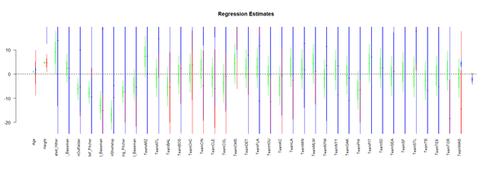
First see the Multiple Linear Regression section, where we discuss linear modeling, review, and demonstrate computing and visualizing the regression-model coefficients (effect-sizes), (fixed-effect) linear model assumptions, examination of residual plots, and independence.
To visualize the Regression-Model coefficients (effect-sizes) we can use the arm package:
#library("arm")
# data <- read.table('01a_data.txt',as.is=T, header=T)
data <- read.table('01a_data.txt',as.is=T, header=T)
attach(data)
df.2 = data.frame(Age, Weight, Height, Position, Team)
lm.2 = lm(Weight ~ Age + Height+ Position + Team, df.2)
lm.3 = lm(Weight ~ Age*Height+ Position*Team, df.2)
lm.4 = lm(Weight ~ Age*Team + Position*Height, df.2)
par (mfrow=c(1,1))
# coefplot(lm.2, xlim=c(-2, 2),  intercept=TRUE)
coefplot(lm.2, vertical=FALSE, col.pts="green")
coefplot(lm.3, vertical=FALSE, add=TRUE, col.pts="red", offset=0.2)
coefplot(lm.3a, vertical=FALSE, add=TRUE, col.pts="black", offset=0.4)
coefplot(lm.4, vertical=FALSE, add=TRUE, col.pts="blue", offset=0.6)
(Fixed-Effect) Linear Model Assumptions
The linear modeling approach (above) is referred to as a linear model, as opposed to another type of model (e.g., non-linear, exponential, etc.) for 2 reasons. First, functional analytic representation of the model involves linear terms of the predictive variables. Second, the model assumptions dictate linear relationships among the covariates and between covariates and response.
Linearity
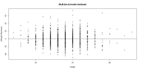
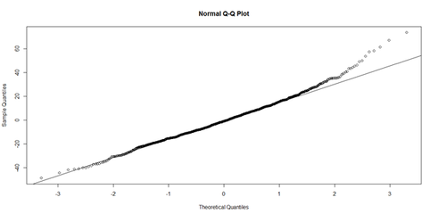
The response variable (Y=Weight, in our case) can be expressed via a linear combination formula of the independent variable (e.g., Height, Age, etc.). If its assumption is invalid, the residual plot may include patterns (e.g., quadratic curve or non-linear trend) indicating another type of model may be appropriate. For instance, the residuals may include a pair of lines when we have dichotomous categorical data. Similarly, the QQ Normal Probability Plot may not be perfectly linear (e.g., S-shaped), which again indicates the distribution of the residuals (observed minus fitted (predicted) values) may not be IID Normal (Gaussian distributed).
This plot shows the age/pitch relationship along with the depiction of the residuals:
# Weight ~ Age + Height + Position + Team + e
# lm.4 = lm(Weight ~ Age.centered + Height+ Position + Team, df.2)
lm.4.res = resid(lm.4)
plot(Height, lm.4.res, ylab="(Weight) Residuals", xlab="Height", main="MLB (lm.4) model residuals")
abline(0, 0)
# Weight ~ Age + Height + Position + Team + e
# lm.4 = lm(Weight ~ Age.centered + Height+ Position + Team, df.2)
# lm.4.res = resid(lm.4)
qqnorm(lm.4.res) 	# A quantile normal plot - good for checking normality
qqline(lm.4.res)
Mind that now, for illustrative purposes, we change the model to (lm.2: Weight ~ Age)!
# lm.2 = lm(Weight ~ Age, df.2)
# calculate residuals and predicted values
lm.2.res = resid(lm.2)
residuals <- signif(lm.2.res, 5)
predicted <- predict(lm.2)
plot(Age, Weight, main="Visualization of the Residuals of Model: Weight ~ Age", xlab="Age", ylab="Weight", pch=19)
abline(lm(Weight ~ Age), col="red")
# plot distances between points and the regression line
segments(Age, Weight, Age, predicted, col="blue")
# add residual-value labels to (Age) points
# install.packages("calibrate")
# library("calibrate", lib.loc="~/R/win-library/3.1")
library(calibrate)
textxy(Age, Weight, residuals, cx=0.7)
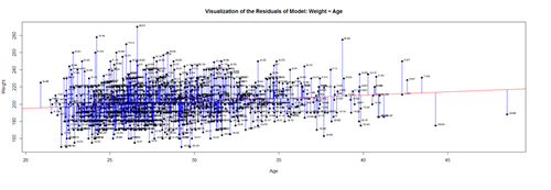
The blue lines indicate the (magnitude of the) residuals and represent the deviations of the observed data points from the model-predicted values (fitted values). The sum of all residuals (positive and negative) is zero, ensured by the least-squares method for estimating the linear model parameters (intercept and slope).
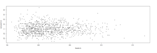
An alternative view is to plot the fitted values (predicted means) on the horizontal line and the residuals, as deviations, on the vertical line.
plot(fitted(lm.2),residuals(lm.2))
Protocols for Rectifying Residual Plots Indicating Nonlinearity
Model may be excluding important fixed effects that interact with fixed effects already accounted for in the model. If new fixed effects are added, the pattern in the residual plot may disappear.
- Variable transformation – Perform a nonlinear transformation of the response, e.g., log, or reciprocal transform. See this SOCR Activity5.
- Perform a nonlinear transformation to explanatory variables. For instance, if Age is related to Weight in a U-shaped way (e.g., quadratic relation), then the model could include Age and Age2 as predictors.
- If residual plots include stripes, then there may be categorical variables playing role, which may necessitate alternative class of models, such as logistic or multinomial models.
Lack of Collinearity
A pair of (linearly) correlated predictors are also called collinear. Suppose Age and Height are correlated (which is certainly to be expected!), then including both as predictors of Weight presents a collinearity problem. In the presence of significant variable collinearity, the interpretation of the model becomes challenging. Depending on which correlated predictors are included in the model, the fixed effects may (incorrectly) become significant or insignificant. Significant findings for these correlated or collinear fixed effects is difficult to interpret as there may be trading-off between the "explanatory power" of the pair of covariates. Multiple predictors that are very similar (linearly correlated) inhibit our ability to decide what plays a big role and what has only marginal impact on the response.
Collinearity may be avoided early during the study-design/data-collection phase of the study to collect fewer fixed effects known to not be linearly correlated. Alternatively, we can selectively include/exclude predictors (e.g., only include in model the most meaningful independent variable and drop the others). Dimensionality reduction methods (e.g., Principal/Independent Component Analyses) also identify (fuse) linearly correlated variables into factors (representing linear combinations transforming several correlated variables into one component variable, which can be used as new fixed effect).
Heteroskedasticity (lack of homoscedasticity)
If the variance of the data is (approximately) stable across the range of the predicted values, then the process is homoscedastic (equal variance assumption). Otherwise, when the homoscedasticity criterion is violated, the process is called heteroskedastic (unequal variances).
Satisfying the homoscedasticity assumption requires the model residuals to roughly have a similar amount of deviation from the predicted values. This can be checked by examining the residual plot.
# lm.2 = lm(Weight ~ Age, df.2)
lm.2.res = resid(lm.2)
plot(Age, lm.2.res, ylab="(Weight) Residuals", xlab="Age", main="MLB (lm.2) model residuals")
abline(0, 0)
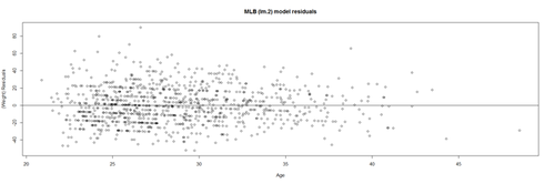
Overall, these data are mostly homoscedastic. A good residual plot essentially looks like a random blob cluster. For instance, using real (simulated) random data, we can see the expectation for the residuals under the linear model assumptions:
plot(rnorm(1000), rbeta(1000, 1,1)-0.5)
abline(0, 0)
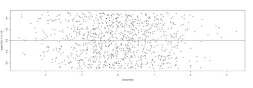
This creates two sets of 1,000 random numbers (x and y axes representing Normal(mean=0,SD=1) and Beta(1,1) distributions, respectively6). Redoing this simulation multiple times and recreating the residual plots will *not* change the appearance of the scatter!
However, there are many situations where the residual plots may show clear heteroskedasticity:
set.seed(11)		# see the random generator with some integer
n <- 256		# define sample size
X <- (1:n)/n           # The set of the predictor X values (uniform steps of 1/n from 0 to 1)
E <- rnorm(n, sd=1)         # A set of *normally distributed* random noise E values
i <- order(runif(n, max=dnorm(E))) # Reorder E, by putting larger errors at the end, on average
Y <- 1 + 5 * X + E[rev(i)]   # Simulate new (observed responses) Y values, X plus "error" `E`.
lm.5 <- lm(Y ~ X)             # Regress `Y` against `X`.
par(mfrow=c(1,3))             # Set up 1 row of 3 plots for drawing the graphs
plot(X,Y, main="Simulated Noisy Data (Y) across time/index", cex=0.8)
abline(coef(lm.5), col="Red")
hist(residuals(lm.5), main="Linear Model Residuals")
plot(predict(lm.5), residuals(lm.5), cex=0.8, main="Residuals vs. Predicted (Heteroskedasticity)")
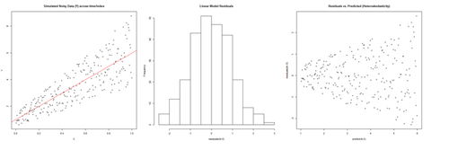
In this example, larger fitted values correspond with larger residuals (the opposite may be true as well). Transforming the data often helps resolve such Heteroskedasticity.
Normality of residuals
The normality of residuals assumption (parametric assumptions) is also important. Linear models may be robust and gracefully handle certain some violations of the normality assumption.
# lm.2 = lm(Weight ~ Age, df.2)
par(mfrow=c(1,2))
hist(residuals(lm.2))
qqnorm(residuals(lm.2))
qqline(lm.2.res, col="red")
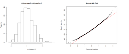
The histogram (left) is relatively bell-shaped and the Q-Q normal probability plot (right) indicates the residuals are mostly on a straight line (suggesting errors (observed-predicted) are similar to a normal distribution). Thus, there is no strong evidence suggesting possible violation of the normality assumption.
Outliers (influential data points)
Data should not include extreme influential points, otherwise the linear model may be heavily biased. Outliers (influential data points) can drastically change the interpretation of model results and inference, similarly to variable collinearity.
The R function dfbeta() computes some of the regression (leave-one-out deletion) diagnostics for linear models and allows us to check for outliers.
Coefficients
Linear mixed effects analyses for scientific inference based on fixed and random effect models, assumptions, and mixed effects logistic regression.
#lm.2 = lm(Weight ~ Age, df.2)
df.results <- dfbeta (lm.2)
head(df.results)
#lm.2 = lm(Weight ~ Age, df.2)
Coefficients:
           Estimate Std. Error t value Pr(>|t|)
(Intercept) 179.6684     4.3418  41.381  < 2e-16 ***
Age           0.7672     0.1494   5.135 3.37e-07 ***
| Intercept | Age | |
| 1 | -0.1654198377 | 0.0051723556 |
| 2 | -0.0690980186 | 0.0026986682 |
| 3 | -0.0139731950 | 0.0007125283 |
| 4 | -0.0284523604 | 0.0010963970 |
| 5 | 0.1803531368 | -0.0069199855 |
| 6 | 0.0001719468 | -0.0008892050 |
For each coefficient of the lm.2 model (intercept, Age, etc.), dfbeta gives the DFbeta values. The first row means that the coefficient for Age (0.7672) has to be adjusted by 0.0051723556 if data point 1 is excluded. In other words, the Age coefficient of the model without the first data point would be -‐0.7723724 (=0.7672 + 0.0051723556). If the slope is negative, DFbeta values are subtracted; if the slope is positive, DFbeta values are added.
Interpretation of large or a small DFbeta values is similarly "open" as the interpretation of p-values (case-specific). However, if the DFbeta value changes, the sign of the coefficient slope, then this data point is an outlier candidate (influential point) that needs special attention. Excluding that 1 point would change the interpretation of the model results.
For small to medium size (n) data, |DFbeta| > 1 is generally suspicious (outlier). For larger datasets, a rule of thumb criterion is |DFbeta| > 2⁄√n
par(mfrow=c(1,1))
plot(df.results, pch=23, bg= 'orange', cex=2, ylab="BFBeta(Weight)")
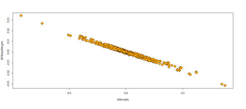
Excluding outliers and reporting results using the reduced data set is not an optimal solution. Running and reporting both the analyses with/without the influential points may be a better strategy. We can exclude influential points when there evidence that these represent technical errors.
Independence
The independence linear model assumption is the most important limitation (which plays role in most statistical tests). Each data point is supposed to be independent from all the others (e.g., observations come from different subjects).
Violations of the independence assumption make the interpretation of the model results impractical. All assumptions are important; however, the independence assumption is critical. Violating independence may inflate the chance of finding spurious effects, bias the results and generate meaningless p‐values.
Independence is mostly a question of the experimental design which is tightly intertwined with the subsequent statistical analyses. When the study design demands collection of more data per subject, repeated measure designs, the data will have (time) dependencies and the appropriate statistical methodologies for interrogating such data involve mixed linear models.
Footnotes
5 http://wiki.socr.umich.edu/index.php/SOCR_EduMaterials_Activities_PowerTransformFamily_Graphs
6 http://socr.umich.edu/html/dist/
See next
- Linear mixed effects analyses where we present scientific inference based on fixed and random effect models, assumptions, and mixed effects logistic regression.
- SOCR Home page: http://www.socr.umich.edu
Translate this page: