SMHS SLR
Contents
[hide]Scientific Methods for Health Sciences - Correlation and Simple Linear Regression (SLR)
Overview
Many scientific applications involve the analysis of relationships between two or more variables involved in studying a process of interest. In this section, we are going to study on the correlations between 2 variables and start with simple linear regressions. Consider the simplest of all situations where Bivariate data (X and Y) are measured for a process and we are interested in determining the association with an appropriate model for the given observations. The first part of this lecture will discuss about correlation and then we are going to talk about SLR to address correlations.
Motivation
The analysis of relationships, if any, between two or more variables involved in the process of interest is widely needed in various studies. We begin with the simplest of all situations where bivariate data (X and Y) are measured for a process and we are interested in determining the association, relation or an appropriate model for these observations (e.g., fitting a straight line to the pairs of (X,Y) data). For example, we measured students of their math scores in the final exam and we want to find out if there is any association between the final score and their participation rate in the math class. Or we are interested to find out if there is any association between weight and lung capacity. Simple linear regression would certainly be a simple way to start and it can address the association very well in simple cases.
Theory
- Correlation: correlation efficient $(-1≤\rho≤1)$ is a measure of linear association or clustering around a line of multivariate data. The main relationship between two variables (X,Y) can be summarized by $(\mu_{X},\sigma_{X})$,$(\mu_{Y},\sigma_{Y})$ and the correlation coefficient denoted by $\rho$=$\rho(X,Y)$.
- The correlation is defined only if both of the standard deviations are finite and are nonzero and it is bounded by -1≤$\rho$≤1.
- If $\rho$=1, perfect positive correlation (straight line relationship between the two variables); if $\rho$=0, no correlation (random cloud scatter), i.e., no linear relation between X and Y; if $\rho$=-1, a perfect negative correlation between the variables.
- $\rho(X,Y)$ $=\frac{cov(X,Y)}{\sigma_{X}\sigma_{Y}}$=$\frac{E((X-μ_{X})(Y-μ_{Y}))}{\sigma_{X}\sigma_{Y}}$=${E(XY)-E(X)E(Y)}\over{\sqrt{E(X^{2})-E^{2}(X)}\sqrt{E(Y^{2})-E^{2}(Y)}},$ where E is the expectation operator, and cov is the covariance. $\mu_{X}=E(X)$,$\sigma_{X}^{2}=E(X^{2})-E^{2}(X),$ and similarly for the second variable, Y, and $cov(X,Y)=E(XY)-E(X)*E(Y)$.
- Sample correlation: replace the unknown expectations and standard deviations by sample mean and sample standard deviation: suppose ${X_{1},X_{2},…,X_{n}}$ and ${Y_{1},Y_{2},…,Y_{n}}$ are bivariate observations of the same process and $(\mu_{X}$,$\sigma_{X})$,$\mu_{Y},\sigma_{Y})$ are the mean and standard deviations for the X and Y measurements respectively. $\rho(x,y)=\frac{\sum x_{i} y_{i}-n\bar{x}\bar{y}}{(n-1)s_{x} s_{y}}$=$\frac{n \sum x_{i} y_{i}-\sum x_{i}\sum y_{i}} {{\sqrt{n\sum x_{i}^{2} -(\sum x_{i})^{2}}} {\sqrt{ n\sum y_{i}^{2}-y_{i})^{2}}}}$; $\rho(x,y)=\frac{\sum(x_{i}-\bar x)(y_{i}-\bar y)}{(n-1)s_{x} s_{y}}$ $=\frac{1}{n-1}$ $\sum$ $\frac{x_{i}-\bar x}{s_{x}}\frac{y_{i}-\bar y}{s_{y}}$, $\bar X$ and $\bar y$ are the sample mean for $X$ and $Y$, $s_{x}$ and $s_{y}$ are the sample standard deviation for $X$ and $Y$.
Hands-on Example
Human weight and height (suppose we took only 6 of the over 25000 observations of human weight and height included in SOCR dataset.
| Subject Index | Height $(x_{i})$ in cm | Weight $(y_{i})$ in kg | $x_{i}-\bar x$ | $y_{i}-\bar y$ | $(x_{i}-\bar x)^{2}$ | $(y_{i}-\bar y)^{2}$ | $(x_{i}-\bar x)(y_{i}-\bar y)$ |
| 1 | 167 | 60 | 6 | 4.6 | 36 | 21.82 | 28.02 |
| 2 | 170 | 64 | 9 | 8.67 | 81 | 75.17 | 78.03 |
| 3 | 160 | 57 | -1 | 1.67 | 1 | 2.79 | -1.67 |
| 4 | 152 | 46 | -9 | -9.33 | 81 | 87.05 | 83.97 |
| 5 | 157 | 55 | -4 | -0.33 | 16 | 0.11 | 1.32 |
| 6 | 160 | 50 | -1 | -5.33 | 1 | 28.41 | 5.33 |
| Total | 966 | 332 | 0 | 0 | 216 | 215.33 | 195 |
$\bar x\frac{966}{6}=161,\bar y=\frac{322}{6}= 55,s_{x}=\sqrt{\frac{216.5}{5}}=6.57, s_{y}=\sqrt{\frac {215.3}{5}}=6.56.$
$\rho(x,y)=\frac{1}{n-1}$ $\sum$ $\frac{x_{i}-\bar x}{s_{x}}\frac{y_{1}-\bar y}{s_{y}}=0.904$
Slope inference
We can conduct inference based on the linear relationship between two quantitative variables by inference on the slope. The basic idea is that we conduct a linear regression of the dependent variable on the predictor suppose they have a linear relationship and we came up with the linear model of y=α+βx+ε, and β is referred to as the true slope of the linear relationship and α represents the intercept of the true linear relationship on y-axis and ε is the random variation. We have talked about the slope in the linear regression, which describes the change in dependent variable y concerned with change in x.
- Test of the significance of the slope β: (1) is there evidence of a real linear relationship which can be done by checking the fit of the residual plots and the initial scatterplots of y vs. x; (2) observations must be independent and the best evidence would be random sample; (3) the variation about the line must be constant, that is the variance of the residuals should be constant which can be checked by the plots of the residuals; (4) the response variable must have normal distribution centered on the line which can be checked with a histogram or normal probability plot.
- Formula we use:$ t=\frac{b-\beta}{SE_{b}}$ , where b stands for the statistic value, $\beta$ is the parameter we are testing on, $SE_{b}$ is the measure of the variation. For the null hypothesis is the $\beta$=0 that is there is no relationship between y and x, so under the null hypothesis, we have the test statistic $t=\frac {b} {SE_{b}}$.
R Examples
Body Fat and Age
Consider a research conducted on see if body fat is associated with age. The data included 18 subjects with the percentage of body fat and the age of the subjects.
| Age | Percentage of Body Fat |
| 23 | 9.5 |
| 23 | 27.9 |
| 27 | 7.8 |
| 27 | 17.8 |
| 39 | 31.4 |
| 41 | 25.9 |
| 45 | 27.4 |
| 49 | 25.2 |
| 50 | 31.1 |
| 53 | 34.7 |
| 53 | 42 |
| 54 | 29.1 |
| 56 | 32.5 |
| 57 | 30.3 |
| 58 | 33 |
| 58 | 33.8 |
| 60 | 41.1 |
| 61 | 34.5 |
The hypothesis tested: $H_{0}:\beta=0$ vs.$H_{a}:\beta\ne0;$ a t-test would be the test we are going to use here given that the data drawn is a random sample from the population.
In R
###
###
## first check the linearity of the relationship using a scatterplot
x <- c(23,23,27,27,39,41,45,49,50,53,53,54,56,57,58,58,60,61)
y <- c(9.5,27.9,7.8,17.8,31.4,25.9,27.4,25.2,31.1,34.7,42,29.1,32.5,30.3,33,33.8,41.1,34.5)
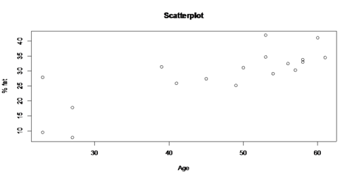
plot(x,y,main='Scatterplot',xlab='Age',ylab='% fat')
cor(x,y)
[1] 0.7920862
The scatterplot shows that there is a linear relationship between x and y, and there is strong positive association of $r=0.7920862$ which further confirms the eye-bow test from the scatterplot about the linear relationship of age and percentage of body fat.
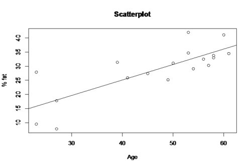
Then we fit a simple linear regression of y on x and draw the scatterplot along with the fitted line:
fit <- lm(y~x)

plot(x,y,main='Scatterplot',xlab='Age',ylab='% fat')

abline(fit)
summary(fit)
Call:
lm(formula = y ~ x)

Residuals:
Min       1Q   Median       3Q      Max
-10.2166  -3.3214  -0.8424   1.9466  12.0753

Coefficients:
Estimate Std. Error t value Pr(>|t|)
(Intercept)   3.2209     5.0762   0.635    0.535
x        0.5480     0.1056   5.191 8.93e-05 \***
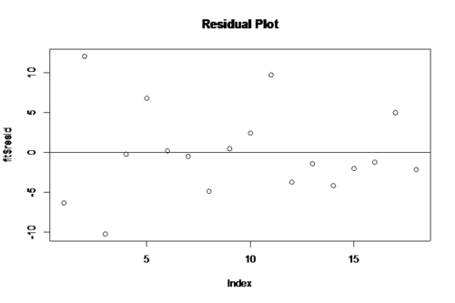
plot(fit$\$ $resid,main='Residual Plot')
abline(y=0)
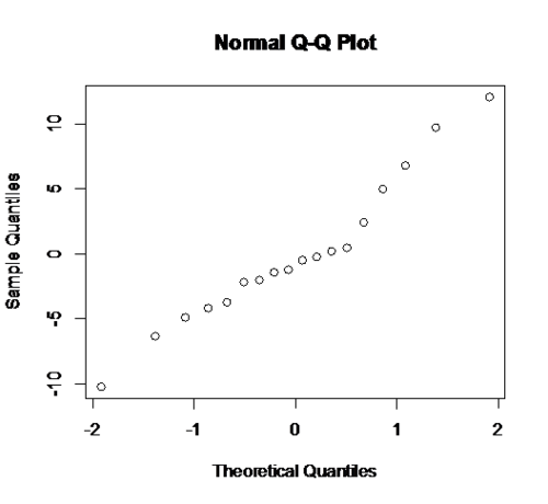
qqnorm(fit$\$ $resid) # check the normality of the residuals
From the residual plot and the QQ plot of residuals we can see that meet the constant variance and normality requirement with no heavy tails and the regression model is reasonable. From the summary of the regression model we have the t-test on the slope has the t value is 5.191 and the p-value is 8.93 e-05. We can reject the null hypothesis of no linear relationship and conclude that is significant linear relationship between age and percentage of body fat at 5% level of significance.
The confidence interval for the parameter tested is $b±t^{*} SE_{b}$, where b is the slope of the least square regression line, $t^{*}$ is the upper $\frac {1-C} {2}$ critical value from the t distribution with degrees of freedom n-2 and $SE_{b}$ is the standard error of the slope.
The standard error of the slope is 0.1056, so we have the 95% CI of the slope is $(0.5480-0.1056*2.12,0.5480+0.1056*2.12)$, that is $(0.324,0.772)$. So, we are 95% confident that the slope will fall in the range between 0.324 and 0.772.
Baseball Example
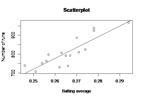
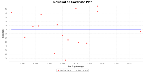
we are studying on a random sample (size 16) of baseball teams and the data show the team’s batting average and the total number of runs scored for the season.
| Batting average | Number of runs scored |
| 0.294 | 968 |
| 0.278 | 938 |
| 0.278 | 925 |
| 0.27 | 887 |
| 0.274 | 825 |
| 0.271 | 810 |
| 0.263 | 807 |
| 0.257 | 798 |
| 0.267 | 793 |
| 0.265 | 792 |
| 0.254 | 764 |
| 0.246 | 740 |
| 0.266 | 738 |
| 0.262 | 31 |
| .251 | 708 |
In R:
x <- c(0.294,0.278,0.278,0.270,0.274,0.271,0.263,0.257,0.267,0.265,0.256,0.254,0.246,0.266,0.262,0.251)
y <- c(968,938,925,887,825,810,807,798,793,792,764,752,740,738,731,708)
cor(x,y)
[1] 0.8654923
The correlation between x and y is 0.8655 which is pretty strong positive correlation. So it would be reasonable to make the assumption of a linear regression model of number of runs scored and the average batting.
fit <- lm(y~x)
summary(fit)
Call:
lm(formula = y ~ x)

Residuals:
*in      1Q  Median      3Q     Max
-74.427 -26.596   1.899  38.156  57.062

Coefficients:
*Estimate Std. Error t value Pr(>|t|)

(Intercept)   -706.2      234.9  -3.006  0.00943 **
x             5709.2      883.1   6.465 1.49e-05 ***
---
Signif. codes:  0 ‘***’ 0.001 ‘**’ 0.01 ‘*’ 0.05 ‘.’ 0.1 ‘ ’ 1
Residual standard error: 40.98 on 14 degrees of freedom

Multiple R-squared: 0.7491,	Adjusted R-squared: 0.7312

F-statistic: 41.79 on 1 and 14 DF,  p-value: 1.486e-05

plot(x,y,main='Scatterplot',xlab='Batting average',ylab='Number of runs')

abline(fit)
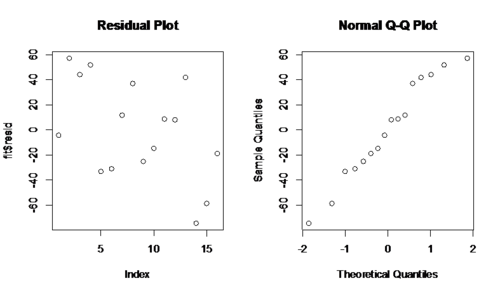
par(mfrow=c(1,2))
plot(fit$\$ $resid,main='Residual Plot')

abline(y=0)

qqnorm(fit$\$ $resid)
The estimated value of the slope is 5709.2, standard error 833.1, t value = 6.465, and the p-value is 1.49 e-05, so we reject the null hypothesis and conclude that there is significant linear relationship between the average batting and the number of runs. We have the 95% CI of the slope is $(5709.2-833.1*2.145,5709.2+833.1*2.145)$, that is $(3922.2,7496.2)$. So, we are 95% confident that the slope will fall in the range between 3922.2 and 7496.2.
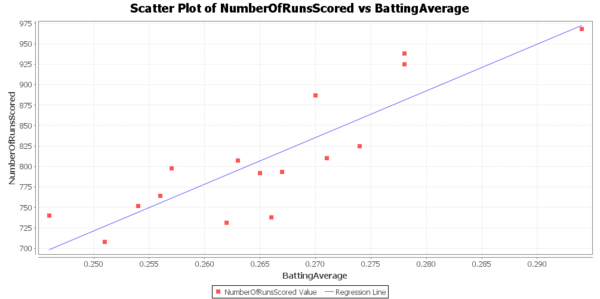
You can also use SOCR SLR Analysis Simple Regression to copy-paste the data in the applet, estimate regression slope and intercept and compute the corresponding statistics and p-values.
Simple Linear Regression Results:
Mean of C1 = 46.33333
Mean of C2 = 28.61111
Regression Line:
C2 = 3.22086 + 0.5479910213243551   C1
Correlation(C1, C2) = .79209
R-Square = .62740
Intercept:
Parameter Estimate: 3.22086
Standard Error:     5.07616
T-Statistics:        .63451
P-Value:            .53472
Slope:
Parameter Estimate: .54799
Standard Error:     .10558
T-Statistics:        5.19053
P-Value:            .00009
Statistical inference on correlation coefficient
Test on $H_{O}:r=\rho$ vs. $H_{a}:r≠\rho$ is the correlation between X and Y. $t_o = \frac{r-\rho}{\sqrt{\frac{1-r^2}{N-2}}}$ with T distribution with $df=N-2$.
Comparing two correlation coefficients: this Fisher’s transformation provides a mechanism to test for comparing two correlation coefficients using Normal distribution. Suppose we have 2 independent paired samples ${(X_{i},Y_{i})}_{i=1}^{n_{1}}$ and ${(U_{j},V_{j} )}_{j=1}^{n_{2}}$ and the $r_{1}=corr(X,Y)$ and $r_{2}=corr(U,V)$ and we are testing $H_{0}: r_{1}=r_{2}$ vs. $H_{a}:r_{1}≠r_{2}$ The Fisher’s transformation for the 2 correlations is defined by $\hat{r}=\frac{1}{2}log_{e}\|\frac{1+r}{1-r}\|$, transforming the two correlation coefficients separately yields $r_{11}=\frac{1}{2}log_{e}\|\frac {1+r_{1}}{1-r_{1}}\|$ and $r_{22}=\frac{1}{2}log_{e}\|\frac{1+r_{22}}{1-r_{22}}\|$. $Z_{0}$ $ =\frac {r_{11}-r_{22}} {\sqrt{\frac{1}{n_{1-3}}-\frac{1}{n_{2-3}}}}$
Note that the hypotheses for the single and double sample inference are $H_{0}:r=0$ vs. $H_{a}:r≠0$ and $H_{0}:r_{1}-r_{2}=0$ vs. $H_{a}:r_{1}-r_{2}≠0$ respectively. And an estimate of the standard deviation of the (Fisher transfored!) correlation is $SD\hat{(r)}=\sqrt{\frac{1}{n-3}}$, thus $r\sim $ $N\bigg (0,\sqrt\frac{1} {n-3}\bigg )$.
Brain Volume Example
The brain volumes (responses) and age (predictors) for 2 cohorts of subjects (Group 1 and Group 2).
| Group1 | Age1 | Volume1 | Group2 | Age2 | Volume2 |
| 1 | 58 | 0.269609 | 2 | 59 | 0.27905 |
| 1 | 55 | 0.277243 | 2 | 50 | 0.262916 |
| 1 | 61 | 0.236264 | 2 | 58 | 0.290697 |
| 1 | 70 | 0.218015 | 2 | 58 | 0.269361 |
| 1 | 38 | 0.287205 | 2 | 61 | 0.268247 |
| 1 | 41 | 0.307387 | 2 | 57 | 0.294204 |
| 1 | 40 | 0.271063 | 2 | 50 | 0.292699 |
| 1 | 25 | 0.307688 | 2 | 38 | 0.273969 |
| 1 | 70 | 0.237811 | 2 | 57 | 0.29049 |
| 1 | 49 | 0.293371 | 2 | 64 | 0.286564 |
| 1 | 56 | 0.252592 | 2 | 71 | 0.257386 |
| 1 | 56 | 0.251349 | 2 | 34 | 0.314958 |
| 1 | 40 | 0.29616 | 2 | 53 | 0.298022 |
| 1 | 50 | 0.249596 | 2 | 53 | 0.269229 |
| 1 | 55 | 0.282721 | 2 | 25 | 0.270634 |
| 1 | 69 | 0.247565 | 2 | 61 | 0.266905 |
We have two independent groups and $Y=volume1$ (response) and $X=age1$ (predictor); $V=volume2$ and $U=age2$, where $n_{1}=27$, $n_{2}=27$. We compute the 2 correlation coefficients: $r_{1}=corr(X,Y)=-0.75338$ and $r_{2}=corr(U,V)=-0.49491.$ Using the Fisher’s transformation we obtain: $r_{11}=\frac{1}{2}log_{e}\|\frac {1+r_{1}}{1-r_{1}}\| = -0.980749 $ and $r_{22}=\frac{1}{2}log_{e}\|\frac{1+r_{2}}{1-r_{2}}\| = -0.5425423,$ $Z_{0}$ $ =\frac {r_{11}-r_{22}} {\sqrt {\frac{1}{n_{1}-3}-\frac{1}{n_{2}-3}}} = 11.517993.$ The corresponding 1-sided p-value =$0.064508$, double-sided p-value =$0.129016$.
Simple linear regression (SLR)
Modeling of the linear relations between two variables using regression analysis. $Y$ is an observed variable and $X$ is specified by the researcher, e.g. $Y$ is hair growth after $X$ months, for individuals at certain does level of hair growth cream; $X$ and $Y$ are both observed variables.
- Estimating the best linear fit: simple linear regression model $Y=a+bX+\varepsilon $ can be estimated using least square, which fits a line minimizing the sums of $ \varepsilon_{l}=\hat y_{l} -y_{i}, \sum_{i=1}^{N} \hat\varepsilon_l^{2}=\sum_{i=1}^{N}(\hat y_{l}-y_{i} )^{2}$, where $ \hat y_{l} = a+bx_{i}$ are observed and predicted values of $Y$ for $x_{i}$.
- Solving for the minimization problem:
- $\hat{b} = \frac {\sum_{i=1}^{N} (x_{i} - \bar{x})(y_{i} - \bar{y}) } {\sum_{i=1}^{N} (x_{i} - \bar{x}) ^2} = \frac {\sum_{i=1}^{N} {(x_{i}y_{i})} - N \bar{x} \bar{y}} {\sum_{i=1}^{N} (x_{i})^2 - N \bar{x}^2} = \rho_{X,Y} \frac {s_y}{s_x},$
- where $\rho_{X,Y}$ is the correlation coefficient.
- $\hat a=\bar y-\hat b\bar x$.
- Properties of the least square line: (1) the line goes through the point of ($\bar{X},\bar{Y}$); (2) the sum of the residuals is equal to zero; (3) the estimates are unbiased, that is their expected values are equal to the real slope and intercept values.
- Regression coefficients inference: when the error terms are normally distributed, then the estimate of the slope coefficient has a normal distribution ith mean equal to $b$ and standard error $SE(\hat b)$ = $s_{\hat b}=\sqrt\frac{1}{N-2}\frac{\sum_{i=1}^{N}\hat\varepsilon_{i}^{2}} {\sum_{i=1}^{N}(x_{i}-\bar x)^{2}}$ To carry out the confidence interval estimating of the slope and intercept of linear model. Given that b follows $\hat b$ follows a T distribution with $N-2$ degrees of freedom, we can calculate the confidence interval for b:$[\hat b-s_{\hat b}t(\frac{\alpha}{2},N-2),\hat b-s_{\hat b}t(\frac{\alpha}{2},N-2)]$ The corresponding test for the regression slope coefficient b is analogously computed $(H_{0}:b=b_{0}$ vs.$H_{a}:b≠b_{0})$ and the test statistic is $t_{0}=\frac{\hat b-b_{0}}s_{\hat b}\sim~T_{df}=N-2$
Earthquake Data Example
- Us the SOCR Data Earthquakes to fit the best linear fit between the longitude and the latitude of the California earthquake since 1900. The SOCR Geomap of these earthquake
- SOCR Google Map Earthquakes shows using the SLR fit to the earthquake data.
Applications
- This article presents the SLR analysis activity in SOCR analysis. It starts with a general introduction to SLR model and then illustrate this method in details with various examples. The article help read results of SLR, make interpretation of the slope and intercept and observe and interpret various data and resulting plots including scatter plots, normal QQ plot and different diagnostic plots such as residual on fit plot.
- This article titled Simple Linear Regression In Medical Research discussed the method of fitting a straight line to data by linear regression and focuses on examples from 36 original articles published in 1978 and 1979. It concluded that investigators need to become better acquainted with residual plots, which give insight into how well the fitted lie models the data, and with confidence bounds for regression lines. Statistical computing package enable investigators to use these techniques easily.
- This article ) presents the r tutorial for simple linear regression. It starts with the fundamental check on the data and comment on the existing patterns found and then fit the linear regression model with the height and weight. It also modified the regression with the Lowess smoothing and talked about the local weighted scatter plot smooth. This article is a comprehensive study on the SLR and correlation in R.
- This articletitled The Probability Plot Correlation Coefficient Test For Normality introduced the normal probability plot correlation coefficient as a test statistic in complete samples for the composite hypothesis of normality. The proposed test statistic is conceptually simple, and is readily extendable to testing non-normal distribution hypotheses. The paper included an empirical power study which shows that the normal probability plot correlation coefficient compared favorably with seven other normal test statistics.
Software
Problems
Example 1: Simple linear correlation and regression in R:
> library(MASS)
> data(cats)
> str(cats)
'data.frame':	144 obs. of  3 variables:
$ Sex: Factor w/ 2 levels "F","M": 1 1 1 1 1 1 1 1 1 1 ...
$ Bwt: num  2 2 2 2.1 2.1 2.1 2.1 2.1 2.1 2.1 ...
$ Hwt: num  7 7.4 9.5 7.2 7.3 7.6 8.1 8.2 8.3 8.5 ...
> summary(cats)
Sex         Bwt             Hwt
F:47   Min.   :2.000   Min.   : 6.30
M:97   1st Qu.:2.300   1st Qu.: 8.95
       Median :2.700   Median :10.10
       Mean   :2.724   Mean   :10.63
       3rd Qu.:3.025   3rd Qu.:12.12
       Max.   :3.900   Max.   :20.50
A positive correlation between two variables X and Y means that if X increases, this will cause the value of Y to increase.
- (a) This is always true.
- (b) This is sometimes true.
- (c) This is never true.
The correlation between working out and body fat was found to be exactly -1.0. Which of the following would not be true about the corresponding scatterplot?
- (a) The slope of the best line of fit should be -1.0.
- (b) All the points would lie along a perfect straight line, with no deviation at all.
- (c) The best fitting line would have a downhill (negative) slope.
- (d) 100% of the variance in body fat can be predicted from workout.
Suppose that the correlation between working out and body fat was found to be exactly -1.0. Which of the following would NOT be true, about the corresponding scatterplot?
- (a) All points would lie along a straight line, with no deviation at all.
- (b) 100% of the variance in body fat can be predicted from the workout.
- (c) The slope of the linear model is -1.0.
- (d) The best fitting line would have a negative slope.
If the correlation coefficient is 0.80, then:
- (a) The explanatory variable is usually less than the response variable.
- (b) The explanatory variable is usually more than the response variable.
- (c) None of the statements are correct.
- (d) Below-average values of the explanatory variable are more often associated with below-average values of the response variable.
- (e) Below-average values of the explanatory variable are more often associated with above-average values of the response variable.
Two different researchers wanted to study the relationship between math anxiety and taking exams. Researcher A measured anxiety with a scale that had a minimum score of 0 and a maximum score of 20, and a final exam that had a minimum score of 0 and a maximum score of 50. He tested 120 students. Researcher B measured anxiety with a scale that had a minimum of 0 and a maximum of 30, and a final exam that had a minimum score of 0 and a maximum score of 35. He tested 60 students. Researcher A found that the coefficient of correlation between a student's math anxiety and his or her score on the final was -0.60. Researcher B found the correlation between a student's math anxiety and his or her score on the final was -0.30.
- (a) The coefficient of correlation for researcher A is twice as strong as the coefficient of correlation for researcher B.
- (b) Based on the study by researcher A one can conclude that high math anxiety is the reason that a lot of the students do not do well in math.
- (c) Given that coefficient of correlation shows the association between standardized scores, one can conclude that for researcher A a greater precentage of the students who have above average anxiety are likely to have below average score on the final.
- (d) Given that the minimum and the maximum values for math and anxiety are so different for the two researchers one cannot compare the coefficient of correlation found by these two researchers.
In the early 1900's when Francis Galton and Karl Pearson measured 1078 pairs of fathers and their grown-up sons, they calculated that the mean height for fathers was 68 inches with deviation of 3 inches. For their sons, the mean height was 69 inches with deviation of 3 inches. (The actual deviations a bit smaller, but we will work with these values to keep the calculations simple.) The correlation coefficient was 0.50. Use the information to calculate the slope of the linear model that predicts the height of the son from the height of the fathers.
- (a) 35.00
- (b) 0.50
- (c) The slope cannot be determined without the actual data
- (d) 3/3 = 1.00
Suppose that wildlife researchers monitor the local alligator population by taking aerial photographs on a regular schedule. They determine that the best fitting linear model to predict weight in pounds from the length of the gators inches is: Weight = -393 + 5.9*Length,with r2 = 0.836. Which of the following statements is true?
- (a) A gator that is about 10 inches above average in length is about 59 pounds above the average weight of these gators.
- (b) The correlation between a gator's length and weight is 0.836.
- (c) The correlation between a gator's height and weight cannot be determined without the actual data.
- (d) The correlation between a gator's height and weight is about -0.914.
Which of the following is NOT a property of the LSR Line?
- (a) The sum of the distances between each point and the LSR Line is minimized.
- (b) The average x value and the average y value lies on the LSR Line
- (c) The sum of squared residuals is minimized
- (d) The sum of the residuals = 0
Suppose that the linear model that predicts fat content in grams from the protein of selected items from Burger Queen menu is: Fat = 6.83 + 0.97*Protein. We learn that there are actually 20 grams of fat in the Chucking burger that has 20 grams of protein. Which of the following statements is true?
- (a) The linear model underestimates the actual fat content and produces a residual of -6.23
- (b) The linear model overestimates the fat content and produces a residual of -6.23
- (c) The linear model underestimates the fat content and produces a residual of -6.23
- (d) The linear model overestimates the fat content and produces a residual of 6.2
Which statement describes the principle of "least squares" that we use in determining the best-fit line?
- (a) The best-fit line minimizes the distances between the observed values and the predicted values.
- (b) The best-fit line minimizes the sum of the squared residuals.
- (c) The best-fit line minimizes the sum of the residuals.
- (d) The best-fit line minimizes the sum of the distances between the actual values and the predicted values.
The scores of midterm and final exams for a random sample of Stats 10 students can be summarized as follows: Mean of midterm score = 36.92; SD of midterm score = 37.79 Mean of final score = 24.71; SD of final score= 25.21 r= 0.978 Choose one answer.
- (a) 23.44
- (b) 0.62
- (c) 25.21
- (d) 35
Which of the following is NOT a property of the Least Squares Regression Line?
- (a) The sum of the distances between each point and the LSR Line is minimized.
- (b) The sum of squared residuals is minimized
- (c) The average x value and the average y value lie on the LSR Line
- (d) The sum of the residuals = 0
Tom and Sue wanted to estimate the average self-esteem score. The true population average for self esteem score is 20. Tom estimates that average by taking a sample of size n and then constructing a confidence interval. What of the following is true? I. The resulting interval will contain 20 II. The 95 percent confidence interval for n = 100 will generally be more narrow than the 95 percent confidence interval for n = 50. III. For n = 100, the 95 percent confidence interval will be wider than the 90 percent confidence interval.
- (a) II only
- (b) III only
- (c) I only
- (d) II and III
A simple random sample of 1000 persons is taken to estimate the percentage of Democrats in a large population. It turns out that 543 of the people in the sample are Democrats. Is the following statement true or false? Explain (51%, 57.5%) is approximately a 95% confidence interval for the sample percentage of democrats.
- (a) False, that is the approximate confidence interval for p. There is no confidence interval for the sample proportion.
- (b) True, we did the computations and those are approximately the numbers for the confidence interval for p.
- (c) True, that is the confidence interval for the sample mean.
- (d) False, the confidence interval for the sample proportion should be smaller than that.
Use the linear model to predict the height of a son whose father's height is 6 feet.
- (a) The son's height = 35 + 0.5(6) inches
- (b) The son's height = 35 + 0.5(72) inches
- (c) The "Regression Effect" states that the son will be a bit taller than his father
- (d) Cannot be determined without the data
A statistician wants to predict Z from Y. He finds that r-squared is 5%.Which one of the following conclusions is correct?
- (a) The coefficient of correlation between Y and Z is 0.05
- (b) Y explains 5% of the variance in Z
- (c) Y is a good predictor of Z
- (d) Z is a good predictor of Y
References
- [Probability_and_statistics_EBook#Chapter_X:_Correlation_and_Regression SOCR COrrelation and Regression Chapter]
- SOCR Home page: http://www.socr.umich.edu
Translate this page:
