SOCR Activity ANOVA FlignerKilleen MeatConsumption
Contents
[hide]- 1 SOCR Educational Materials - Activities - SOCR Meat Consumption Activity – ANOVA assumptions about the variance homogeneity Activity
- 2 Motivation and Goals
- 3 Summary
- 4 Data
- 5 Exploratory data analyses (EDA)
- 6 Quantitative data analysis (QDA)
- 7 Conclusions
- 8 Practice problems
- 9 See also
- 10 References
SOCR Educational Materials - Activities - SOCR Meat Consumption Activity – ANOVA assumptions about the variance homogeneity Activity
Motivation and Goals
In many developed countries, when people imagine their next meal, they focus on one specific part: the meat. That choice of meat, however, varies from country to country due to the popularity and availability of various domesticated animals. Furthermore, the amount of meat eaten has a surprising degree of variability across time, cultures and geographic regions.
The following activity will study the effects of that variance on the statistical analyses. Specifically, we will consider how deviations from homoscedasticity (also known as equivalence of variance or variance homogeneity) can lead to making some incomplete or even incorrect conclusions. To do so, we will employ the Fligner-Killeen method to analyze some real meet consumption data.
Summary
This activity uses a reduced version of the open-source meat-consumption dataset. All data comes from the US Census Bureau.
This dataset summarizes the meat consumption, by animal type, of various countries (the European Union (EU) is being treated as a single country in this case). For simplicity, records from countries that did provide consumption measures for all meat types and all years were removed from the data set.
Data
Data Description
- Number of cases: 147
- Variables
- Country: The country or world region in question
- Brazil
- China
- European Union
- Japan
- Mexico
- Russia
- United States
- Meat: The type of meat
- Beef
- Pork
- Poultry
- Years Represented (2000 – 2006)
- Country: The country or world region in question
- Values are in thousands of metric tons
Data Summaries
Chicken/Poultry
| Year | Brazil | China | Europe | Japan | Mexico | Russia | UnitedStates | YearAverage | YearSD |
|---|---|---|---|---|---|---|---|---|---|
| 2000 | 5110 | 9393 | 6934 | 1772 | 2163 | 1320 | 11474 | 5452.286 | 3990.459 |
| 2001 | 5341 | 9237 | 7359 | 1797 | 2311 | 1588 | 11558 | 5598.714 | 3942.57 |
| 2002 | 5873 | 9556 | 7417 | 1830 | 2424 | 1697 | 12270 | 5866.714 | 4134.211 |
| 2003 | 5742 | 9963 | 7312 | 1841 | 2627 | 1680 | 12540 | 5957.857 | 4234.565 |
| 2004 | 5992 | 9931 | 7280 | 1713 | 2713 | 1675 | 13080 | 6054.857 | 4379.591 |
| 2005 | 6612 | 10088 | 7596 | 1880 | 2871 | 2139 | 13430 | 6373.714 | 4388.111 |
| 2006 | 6853 | 10371 | 7380 | 1908 | 3005 | 2382 | 13754 | 6521.857 | 4448.974 |
| Country_Average | 5931.857 | 9791.286 | 7325.429 | 1820.143 | 2587.714 | 1783 | 12586.57 | ||
| Country_SD | 629.6543 | 407.0908 | 200.4826 | 66.03895 | 304.2404 | 357.6777 | 886.5564 |
Pork
| Year | Brazil | China | Europe | Japan | Mexico | Russia | UnitedStates | YearAverage | YearSD |
|---|---|---|---|---|---|---|---|---|---|
| 2000 | 1827 | 40378 | 19242 | 2228 | 1252 | 2019 | 8455 | 10771.57 | 14570.99 |
| 2001 | 1919 | 41829 | 19317 | 2268 | 1298 | 2076 | 8389 | 11013.71 | 15049.33 |
| 2002 | 1975 | 43238 | 19746 | 2377 | 1349 | 2453 | 8685 | 11403.29 | 15502.7 |
| 2003 | 1957 | 45054 | 20043 | 2373 | 1423 | 2420 | 8816 | 11726.57 | 16145.49 |
| 2004 | 1979 | 46648 | 19773 | 2562 | 1556 | 2337 | 8817 | 11953.14 | 16648.16 |
| 2005 | 1949 | 49703 | 19768 | 2507 | 1556 | 2476 | 8669 | 12375.43 | 17714.83 |
| 2006 | 2191 | 51809 | 20015 | 2450 | 1580 | 2637 | 8640 | 12760.29 | 18438.64 |
| Country_Average | 1971 | 45522.71 | 19700.57 | 2395 | 1430.571 | 2345.429 | 8638.714 | ||
| Country_SD | 110 | 4159.521 | 312.355 | 121.3013 | 135.3808 | 223.0148 | 164.5121 |
Beef
| Year | Brazil | China | Europe | Japan | Mexico | Russia | UnitedStates | YearAverage | YearSD |
|---|---|---|---|---|---|---|---|---|---|
| 2000 | 6102 | 5284 | 8106 | 1585 | 2309 | 2246 | 12502 | 5447.714 | 3922.316 |
| 2001 | 6191 | 5434 | 7658 | 1419 | 2341 | 2400 | 12351 | 5399.143 | 3835.093 |
| 2002 | 6437 | 5818 | 8187 | 1319 | 2409 | 2450 | 12737 | 5622.429 | 4016.753 |
| 2003 | 6273 | 6274 | 8315 | 1366 | 2308 | 2378 | 12340 | 5607.714 | 3933.847 |
| 2004 | 6400 | 6703 | 8292 | 1182 | 2368 | 2308 | 12667 | 5702.857 | 4077.861 |
| 2005 | 6774 | 7026 | 8194 | 1200 | 2419 | 2503 | 12663 | 5825.571 | 4056.693 |
| 2006 | 6939 | 7395 | 8270 | 1173 | 2509 | 2370 | 12830 | 5926.571 | 4148.408 |
| Country_Average | 6445.143 | 6276.286 | 8146 | 1320.571 | 2380.429 | 2379.286 | 12584.29 | ||
| Country_SD | 307.1685 | 806.2036 | 226.9295 | 151.2138 | 71.75388 | 85.31259 | 190.4396 |
Raw Dataset
| Country | Meat | 2000 | 2001 | 2002 | 2003 | 2004 | 2005 | 2006 |
|---|---|---|---|---|---|---|---|---|
| Brazil | Beef | 6102 | 6191 | 6437 | 6273 | 6400 | 6774 | 6939 |
| Brazil | Pork | 1827 | 1919 | 1975 | 1957 | 1979 | 1949 | 2191 |
| Brazil | Poultry | 5110 | 5341 | 5873 | 5742 | 5992 | 6612 | 6853 |
| China | Beef | 5284 | 5434 | 5818 | 6274 | 6703 | 7026 | 7395 |
| China | Pork | 40378 | 41829 | 43238 | 45054 | 46648 | 49703 | 51809 |
| China | Poultry | 9393 | 9237 | 9556 | 9963 | 9931 | 10088 | 10371 |
| EuropeanUnion | Beef | 8106 | 7658 | 8187 | 8315 | 8292 | 8194 | 8270 |
| EuropeanUnion | Pork | 19242 | 19317 | 19746 | 20043 | 19773 | 19768 | 20015 |
| EuropeanUnion | Poultry | 6934 | 7359 | 7417 | 7312 | 7280 | 7596 | 7380 |
| Japan | Beef | 1585 | 1419 | 1319 | 1366 | 1182 | 1200 | 1173 |
| Japan | Pork | 2228 | 2268 | 2377 | 2373 | 2562 | 2507 | 2450 |
| Japan | Poultry | 1772 | 1797 | 1830 | 1841 | 1713 | 1880 | 1908 |
| Mexico | Beef | 2309 | 2341 | 2409 | 2308 | 2368 | 2419 | 2509 |
| Mexico | Pork | 1252 | 1298 | 1349 | 1423 | 1556 | 1556 | 1580 |
| Mexico | Poultry | 2163 | 2311 | 2424 | 2627 | 2713 | 2871 | 3005 |
| Russia | Beef | 2246 | 2400 | 2450 | 2378 | 2308 | 2503 | 2370 |
| Russia | Pork | 2019 | 2076 | 2453 | 2420 | 2337 | 2476 | 2637 |
| Russia | Poultry | 1320 | 1588 | 1697 | 1680 | 1675 | 2139 | 2382 |
| UnitedStates | Beef | 12502 | 12351 | 12737 | 12340 | 12667 | 12663 | 12830 |
| UnitedStates | Pork | 8455 | 8389 | 8685 | 8816 | 8817 | 8669 | 8640 |
| UnitedStates | Poultry | 11474 | 11558 | 12270 | 12540 | 13080 | 13430 | 13754 |
Exploratory data analyses (EDA)
In the following analysis, we will aim to perform an analysis of variance (ANOVA) to compare the meat consumption amounts between different countries and/or across time. Note that the data points for each country-meat type combination are from the various years. Typically, we would expect the amount not to change between the years (especially in this 7-year timespan). Even if it did, in assuming homoscedasticity, we are making the assumption that any increase or decrease is constant between countries. Applying the Fligner-Killeen test will help us decide if this assumption is valid. Look at the bar graphs listed below and note which of them seem to vary more than the others between the years.


Quantitative data analysis (QDA)
ANOVA
Open the SOCR ANOVA-Two Way applet (requires Java-enabled browser). For the following analyses, we will focus on the data for Beef consumption. Let us test to see if different countries eat different amounts of beef. Usually when we compare a set of groups as this one, we would use a one-way ANOVA (comparing the seven countries). To run this test, open up the one-way ANOVA analysis in the SOCR Analyses Applet in a java-enabled browser. It should be the default setting when you open up the page:

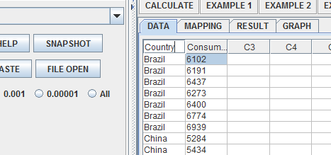
Now, prepare your dataset (it will be the Beef table from the above summary tables). We will be treating the yearly results as being our sample’s data points, attempting to capture the overall population consumption. This seems reasonable; the average meet consumption of a country should not change that much in a seven-year timespan.
Once you have rearranged your dataset for use in the ANOVA applet (if you do not know what it should look like, try considering one of the SOCR ANOVA tutorials). It should look like this in the applet data screen:

Rename your column headers to define the independent and dependent variables.

Click on the mapping tab, and assign your independent and dependent variables appropriately:

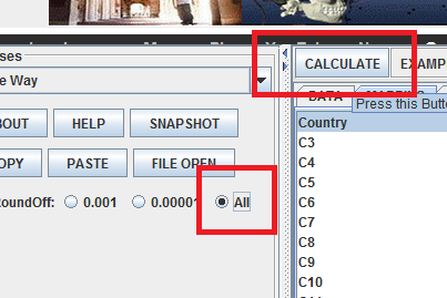
Set your precision to all, then click calculate:

The following results should appear in the Results tab:
- Sample Size = 49
- Independent Variable = Country
- Dependent Variable = Consumption
- Results of One-Way Analysis of Variance:
- Standard 1-Way ANOVA Table
| VarianceSource | DF | RSS | MSS | F-Statistics | P-value |
|---|---|---|---|---|---|
| TreatmentEffect(B/w_Groups) | 6 | 668292765.43 | 111382127.57 | 898.89 | < 1E-15 |
| Error | 42 | 5204240.57 | 123910.48 | ||
| Total | 48 | 673497006.00 |
- Model:
- Degrees of Freedom = 6
- Residual Sum of Squares = 668292765.43
- Mean Square Error = 111382127.57
- Error:
- Degrees of Freedom = 42
- Residual Sum of Squares = 5204240.57
- Mean Square Error = 123910.49
- Corrected Total:
- Degrees of Freedom = 48
- Residual Sum of Squares = 673497006.00
- F-Value = 898.89
- P-Value = < 1E-15
- R-Square = 0.99
Fligner-Killeen Analysis
Note our extremely low p-value. The results of our one-way ANOVA reject the null hypothesis that these countries do not differ in terms of beef consumption. This shouldn’t surprise anyone. Even a third grader could have made that decision after looking at the summary table, or the earlier EDA graphs. Besides, the data represents total volume of meat consumption, whereas the populations of these countries are vastly different, and a per-capita meat consumption analysis may be more appropriate in this case.
However, let’s say that you find a book that claims, using the results of your ANOVA as proof, that “China consumes more beef than any country other than the United States”. That book is saying that these populations are significantly different in terms of their beef consumption. Is this claim justified by the ANOVA analysis above? Going through the assumptions of the ANOVA test, remember that the different levels must follow homoscedasticity (equivalence of variance). If two populations are significantly far from this assumption, then they should be compared using ANOVA. An alternative statistical test needs to be applied (e.g., Kruskal-Wallis test).
To test for homoscedacity, we will use the Fligner-Killeen test, which is a non-parametric test that doesn’t assume normality. This is important, considering that we have a rather limited data set (only seven points, one for each year) and the data may not be normally distributed. Use the tab to find the Fligner-Killeen analysis in the SOCR Analyses Applet in a java-enabled browser:

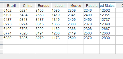
Next, copy and paste your data into the spreadsheet using the paste button built into the applet. The data copied here is from the Beef summary table (excluding the marginal means). Note that we are treating the cases within each country (one for each year) as the data points. When trends take many years to happen, we can assume that, within a short timespan (such as the 7 years captured here), each year serves as estimates of a generally unchanging population value for that country.

Re-name the data headers to the country names, our levels for this comparison.

Click on the mapping tap and add all of the country names to the next tab.

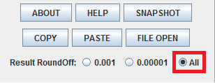
Finally, select the precision setting “All.” This will display the maximum number of decimal numbers. Afterwards, click “CALCULATE”:

The following results text should appear on the screen:
- Group Brazil
- median = 6400.0
- Group China
- median = 6274.0
- Group Europe
- median = 8194.0
- Group Japan
- median = 1319.0
- Group Mexico
- median = 2368.0
- Group Russia
- median = 2378.0
- Group United States
- median = 12663.0
- Total Size = 49
- Total Mean Score = .784
- Total Variance = .323
- Degrees of Freedom = 6
- Chi-Square Statistic = 19.421
- P-Value = .004
The result from the Fligner-Killeen test (for variance homogeneity) yields a rather small p-value (0.004). Assuming α = 0.05, we would rejects the null hypothesis of equal variances between countries. Therefore, we should be wary of continuing with a standard (parametric) Analysis of Variance (ANOVA). Looking back at the data, it is easy to see why.
Conclusions
Note, for example, that in the data for the Chinese consumption of beef, the values are steadily rising between the years. In our ANOVA, we had made an assumption, that the overall consumption would not follow a set pattern between the years, allowing us to treat them as sample points. This results in a much different variance between the groups. Therefore, it would be incorrect to use our previous conclusion from the ANOVA that “these countries have different population values for meat consumption” without a qualifier of the date range that we were sampling within. Note that without this analysis, you might have missed the trend in Chinese beef consumption—which might be worth studying in its own right.
We can also think about this from a more mathematical perspective. This brings up the fundamental definition of Analysis of Variance, in which we are trying to keep constant the within-group variance of each of our levels (in this case, countries). If we ignore homoscedasticity, from the viewpoint of the algebra involved, we are essentially comparing completely unrelated populations.
Just because the assumptions of ANOVA are not satisfied, we should not give up on this data set. Without the results of the Fligner-Killeen, we may have missed the effects of time on meat consumption, an effect that warrants is own investigation. In such situations, the use of non-parametric alternatives to ANOVA may be appropriate (e.g., Kruskal-Wallis test).
Practice problems
- Run this same analysis for the pork and poultry datasets. Interpret any conclusions as shown above.
- Practice running a one-way ANOVA, excluding the data from China and Japan.
- “Turn” the beef data set around, and run this Fligner-Killeen test between the year groups. Interpret the conclusion you find. Why is this same/different to the result from the above example?
See also
References
- Meat Consumption by Type and Country (2006). U.S. Department of Agriculture, Foreign Agricultural Service, Livestock, and Poultry.
"-----
Translate this page: